
8300INTR.DOC TI-83 Intl English, Title Page Bob Fedorisko Revised: 02/19/01 2:32 PM Printed: 02/21/01 9:05
AM Page iii of 8
TI-83
GRAPHING CALCULATOR
GUIDEBOOK
TI-GRAPH LINK, Calculator-Based Laboratory, CBL, CBL 2, Calculator-Based Ranger, CBR,
Constant Memory, Automatic Power Down, APD, and EOS are trademarks of Texas
Instruments Incorporated.
IBM is a registered trademark of International Business Machines Corporation.
Macintosh is a registered trademark of Apple Computer, Inc.
Windows is a registered trademark of Microsoft Corporation.
© 1996, 2000, 2001 Texas Instruments Incorporated.

8300INTR.DOC TI-83 Intl English, Title Page Bob Fedorisko Revised: 02/19/01 11:26 AM Printed: 02/19/01 1:46
PM Page iv of 8
Texas Instruments makes no warranty, either expressed or
implied, including but not limited to any implied warranties of
merchantability and fitness for a particular purpose, regarding any
programs or book materials and makes such materials available
solely on an “as-is” basis.
In no event shall Texas Instruments be liable to anyone for special,
collateral, incidental, or consequential damages in connection with
or arising out of the purchase or use of these materials, and the
sole and exclusive liability of Texas Instruments, regardless of the
form of action, shall not exceed the purchase price of this
equipment. Moreover, Texas Instruments shall not be liable for any
claim of any kind whatsoever against the use of these materials by
any other party.
This equipment has been tested and found to comply with the
limits for a Class B digital device, pursuant to Part 15 of the FCC
rules. These limits are designed to provide reasonable protection
against harmful interference in a residential installation. This
equipment generates, uses, and can radiate radio frequency energy
and, if not installed and used in accordance with the instructions,
may cause harmful interference with radio communications.
However, there is no guarantee that interference will not occur in
a particular installation.
If this equipment does cause harmful interference to radio or
television reception, which can be determined by turning the
equipment off and on, you can try to correct the interference by
one or more of the following measures:
• Reorient or relocate the receiving antenna.
• Increase the separation between the equipment and receiver.
• Connect the equipment into an outlet on a circuit different
from that to which the receiver is connected.
• Consult the dealer or an experienced radio/television
technician for help.
Caution: Any changes or modifications to this equipment not
expressly approved by Texas Instruments may void your authority
to operate the equipment.
Important
US FCC
Information
Concerning
Radio Frequency
Interference

Introduction iii
8300INTR.DOC TI-83 Intl English, Title Page Bob Fedorisko Revised: 02/19/01 11:26 AM Printed: 02/19/01 1:46
PM Page iii of 8
This manual describes how to use the TI
.
83 Graphing Calculator. Getting
Started is an overview of TI
.
83 features. Chapter 1 describes how the TI
.
83
operates. Other chapters describe various interactive features. Chapter 17
shows how to combine these features to solve problems.
TI
-
83 Keyboard
..........................................
2
TI
-
83 Menus
.............................................
4
First Steps
...............................................
5
Entering a Calculation: The Quadratic Formula
..........
6
Converting to a Fraction: The Quadratic Formula
........
7
Displaying Complex Results: The Quadratic Formula
....
8
Defining a Function: Box with Lid
.......................
9
Defining a Table of Values: Box with Lid
.................
10
Zooming In on the Table: Box with Lid
...................
11
Setting the Viewing Window: Box with Lid
...............
12
Displaying and Tracing the Graph: Box with Lid
.........
13
Zooming In on the Graph: Box with Lid
..................
15
Finding the Calculated Maximum: Box with Lid
..........
16
Other TI
-
83 Features
.....................................
17
Turning On and Turning Off the TI
-
83
....................
1
-
2
Setting the Display Contrast
.............................
1
-
3
The Display
..............................................
1
-
4
Entering Expressions and Instructions
...................
1
-
6
TI
-
83 Edit Keys
..........................................
1
-
8
Setting Modes
...........................................
1
-
9
Using TI
-
83 Variable Names
.............................
1
-
13
Storing Variable Values
..................................
1
-
14
Recalling Variable Values
................................
1
-
15
ENTRY
(Last Entry) Storage Area
........................
1
-
16
Ans
(Last Answer) Storage Area
.........................
1
-
18
TI
-
83 Menus
.............................................
1
-
19
VARS
and
VARS Y
.
VARS
Menus
.........................
1
-
21
Equation Operating System (EOS
é
)
.....................
1
-
22
Error Conditions
.........................................
1
-
24
Table of Contents
Getting Started:
Do This First!
Chapter 1:
Operating the
TI-83

iv Introduction
8300INTR.DOC TI-83 Intl English, Title Page Bob Fedorisko Revised: 02/19/01 11:26 AM Printed: 02/19/01 1:46
PM Page iv of 8
Getting Started: Coin Flip
................................
2
-
2
Keyboard Math Operations
..............................
2
-
3
MATH
Operations
........................................
2
-
5
Using the Equation Solver
...............................
2
-
8
MATH NUM
(Number) Operations
........................
2
-
13
Entering and Using Complex Numbers
...................
2
-
16
MATH CPX
(Complex) Operations
.......................
2
-
18
MATH PRB
(Probability) Operations
.....................
2
-
20
ANGLE
Operations
.......................................
2
-
23
TEST
(Relational) Operations
............................
2
-
25
TEST LOGIC
(Boolean) Operations
......................
2
-
26
Getting Started: Graphing a Circle
.......................
3
-
2
Defining Graphs
.........................................
3
-
3
Setting the Graph Modes
.................................
3
-
4
Defining Functions
......................................
3
-
5
Selecting and Deselecting Functions
.....................
3
-
7
Setting Graph Styles for Functions
.......................
3
-
9
Setting the Viewing Window Variables
...................
3
-
11
Setting the Graph Format
................................
3
-
13
Displaying Graphs
.......................................
3
-
15
Exploring Graphs with the Free-Moving Cursor
..........
3
-
17
Exploring Graphs with
TRACE
...........................
3
-
18
Exploring Graphs with the
ZOOM
Instructions
...........
3
-
20
Using
ZOOM MEMORY
..................................
3
-
23
Using the
CALC
(Calculate) Operations
..................
3
-
25
Getting Started: Path of a Ball
...........................
4
-
2
Defining and Displaying Parametric Graphs
..............
4
-
4
Exploring Parametric Graphs
............................
4
-
7
Getting Started: Polar Rose
..............................
5
-
2
Defining and Displaying Polar Graphs
...................
5
-
3
Exploring Polar Graphs
..................................
5
-
6
Chapter 2:
Math, Angle, and
Test Operations
Chapter 3:
Function
Graphing
Chapter 4:
Parametric
Graphing
Chapter 5:
Polar Graphing

Introduction v
8300INTR.DOC TI-83 Intl English, Title Page Bob Fedorisko Revised: 02/19/01 11:26 AM Printed: 02/19/01 1:46
PM Page v of 8
Getting Started: Forest and Trees
........................
6
-
2
Defining and Displaying Sequence Graphs
...............
6
-
3
Selecting Axes Combinations
............................
6
-
8
Exploring Sequence Graphs
..............................
6
-
9
Graphing Web Plots
......................................
6
-
11
Using Web Plots to Illustrate Convergence
...............
6
-
12
Graphing Phase Plots
....................................
6
-
13
Comparing TI
-
83 and TI
.
82 Sequence Variables
..........
6
-
15
Keystroke Differences Between TI
-
83 and TI
-
82
.........
6
-
16
Getting Started: Roots of a Function
.....................
7
-
2
Setting Up the Table
.....................................
7
-
3
Defining the Dependent Variables
........................
7
-
4
Displaying the Table
.....................................
7
-
5
Getting Started: Drawing a Tangent Line
.................
8
-
2
Using the
DRAW
Menu
...................................
8
-
3
Clearing Drawings
.......................................
8
-
4
Drawing Line Segments
..................................
8
-
5
Drawing Horizontal and Vertical Lines
...................
8
-
6
Drawing Tangent Lines
..................................
8
-
8
Drawing Functions and Inverses
.........................
8
-
9
Shading Areas on a Graph
...............................
8
-
10
Drawing Circles
..........................................
8
-
11
Placing Text on a Graph
.................................
8
-
12
Using Pen to Draw on a Graph
...........................
8
-
13
Drawing Points on a Graph
..............................
8
-
14
Drawing Pixels
..........................................
8
-
16
Storing Graph Pictures (
Pic
)
.............................
8
-
17
Recalling Graph Pictures (
Pic
)
...........................
8
-
18
Storing Graph Databases (
GDB
)
.........................
8
-
19
Recalling Graph Databases (
GDB
)
.......................
8
-
20
Getting Started: Exploring the Unit Circle
................
9
-
2
Using Split Screen
.......................................
9
-
3
Horiz
(Horizontal) Split Screen
...........................
9
-
4
G
-
T
(Graph-Table) Split Screen
..........................
9
-
5
TI
.
83 Pixels in
Horiz
and
G
-
T
Modes
.....................
9
-
6
Chapter 6:
Sequence
Graphing
Chapter 7:
Tables
Chapter 8:
DRAW
Operations
Chapter 9:
Split Screen

vi Introduction
8300INTR.DOC TI-83 Intl English, Title Page Bob Fedorisko Revised: 02/19/01 11:26 AM Printed: 02/19/01 1:46
PM Page vi of 8
Getting Started: Systems of Linear Equations
............
10
-
2
Defining a Matrix
........................................
10
-
3
Viewing and Editing Matrix Elements
....................
10
-
4
Using Matrices with Expressions
........................
10
-
7
Displaying and Copying Matrices
........................
10
-
8
Using Math Functions with Matrices
.....................
10
-
9
Using the
MATRX MATH
Operations
.....................
10
-
12
Getting Started: Generating a Sequence
..................
11
-
2
Naming Lists
.............................................
11
-
3
Storing and Displaying Lists
.............................
11
-
4
Entering List Names
.....................................
11
-
6
Attaching Formulas to List Names
.......................
11
-
7
Using Lists in Expressions
...............................
11
-
9
LIST OPS
Menu
..........................................
11
-
10
LIST MATH
Menu
........................................
11
-
17
Getting Started: Pendulum Lengths and Periods
.........
12
-
2
Setting up Statistical Analyses
...........................
12
-
10
Using the Stat List Editor
................................
12
-
11
Attaching Formulas to List Names
.......................
12
-
14
Detaching Formulas from List Names
....................
12
-
16
Switching Stat List Editor Contexts
......................
12
-
17
Stat List Editor Contexts
.................................
12
-
18
STAT EDIT
Menu
........................................
12
-
20
Regression Model Features
..............................
12
-
22
STAT CALC
Menu
........................................
12
-
24
Statistical Variables
......................................
12
-
29
Statistical Analysis in a Program
.........................
12
-
30
Statistical Plotting
.......................................
12
-
31
Statistical Plotting in a Program
.........................
12
-
37
Getting Started: Mean Height of a Population
............
13
-
2
Inferential Stat Editors
...................................
13
-
6
STAT TESTS
Menu
......................................
13
-
9
Inferential Statistics Input Descriptions
..................
13
-
26
Test and Interval Output Variables
.......................
13
-
28
Distribution Functions
...................................
13
-
29
Distribution Shading
.....................................
13
-
35
Chapter 10:
Matrices
Chapter 11:
Lists
Chapter 12:
Statistics
Chapter 13:
Inferential
Statistics and
Distributions

Introduction vii
8300INTR.DOC TI-83 Intl English, Title Page Bob Fedorisko Revised: 02/19/01 11:26 AM Printed: 02/19/01 1:46
PM Page vii of 8
Getting Started: Financing a Car
.........................
14
-
2
Getting Started: Computing Compound Interest
..........
14
-
3
Using the
TVM Solver
....................................
14
-
4
Using the Financial Functions
...........................
14
-
5
Calculating Time Value of Money (
TVM
)
.................
14
-
6
Calculating Cash Flows
..................................
14
-
8
Calculating Amortization
................................
14
-
9
Calculating Interest Conversion
..........................
14
-
12
Finding Days between Dates/Defining Payment Method
.....
14
-
13
Using the
TVM
Variables
.................................
14
-
14
Browsing the TI
-
83
CATALOG
...........................
15
-
2
Entering and Using Strings
...............................
15
-
3
Storing Strings to String Variables
.......................
15
-
4
String Functions and Instructions in the
CATALOG
......
15
-
6
Hyperbolic Functions in the
CATALOG
..................
15
-
10
Getting Started: Volume of a Cylinder
....................
16
-
2
Creating and Deleting Programs
.........................
16
-
4
Entering Command Lines and Executing Programs
......
16
-
5
Editing Programs
........................................
16
-
6
Copying and Renaming Programs
........................
16
-
7
PRGM CTL
(Control) Instructions
.......................
16
-
8
PRGM I/O
(Input/Output) Instructions
...................
16
-
16
Calling Other Programs as Subroutines
..................
16
-
22
Comparing Test Results Using Box Plots
................
17
-
2
Graphing Piecewise Functions
...........................
17
-
4
Graphing Inequalities
....................................
17
-
5
Solving a System of Nonlinear Equations
................
17
-
6
Using a Program to Create the Sierpinski Triangle
.......
17
-
7
Graphing Cobweb Attractors
............................
17
-
8
Using a Program to Guess the Coefficients
...............
17
-
9
Graphing the Unit Circle and Trigonometric Curves
......
17
-
10
Finding the Area between Curves
........................
17
-
11
Using Parametric Equations: Ferris Wheel Problem
......
17
-
12
Demonstrating the Fundamental Theorem of Calculus
...
17
-
14
Computing Areas of Regular N-Sided Polygons
..........
17
-
16
Computing and Graphing Mortgage Payments
...........
17
-
18
Chapter 14:
Financial
Functions
Chapter 15:
CATALOG,
Strings,
Hyperbolic
Functions
Chapter 16:
Programming
Chapter 17:
Applications

viii Introduction
8300INTR.DOC TI-83 Intl English, Title Page Bob Fedorisko Revised: 02/19/01 11:26 AM Printed: 02/19/01 1:46
PM Page viii of 8
Checking Available Memory
.............................
18
-
2
Deleting Items from Memory
............................
18
-
3
Clearing Entries and List Elements
......................
18
-
4
Resetting the TI
.
83
......................................
18
-
5
Getting Started: Sending Variables
.......................
19
-
2
TI
-
83
LINK
...............................................
19
-
3
Selecting Items to Send
..................................
19
-
4
Receiving Items
..........................................
19
-
5
Transmitting Items
.......................................
19
-
6
Transmitting Lists to a TI
-
82
.............................
19
-
8
Transmitting from a TI
-
82 to a TI
-
83
.....................
19
-
9
Backing Up Memory
.....................................
19
-
10
Table of Functions and Instructions
.....................
A
-
2
Menu Map
...............................................
A
-
39
Variables
................................................
A
-
49
Statistical Formulas
.....................................
A
-
50
Financial Formulas
......................................
A
-
54
Battery Information
......................................
B
-
2
In Case of Difficulty
.....................................
B
-
4
Error Conditions
.........................................
B
-
5
Accuracy Information
....................................
B
-
10
Support and Service Information
.........................
B
-
12
Warranty Information
....................................
B
-
13
Chapter 18:
Memory
Management
Chapter 19:
Communication
Link
Appendix A:
Tables and
Reference
Information
Appendix B:
General
Information
Index
Getting Started 1
8300GETM.DOC TI-83 international English Bob Fedorisko Revised: 02/19/01 11:06 AM Printed: 02/19/01 11:06
AM Page 1 of 18
Gettin
g
Started:
Do This First!
TI
-
83 Keyboard
..........................................
2
TI
-
83 Menus
.............................................
4
First Steps
...............................................
5
Entering a Calculation: The Quadratic Formula
..........
6
Converting to a Fraction: The Quadratic Formula
........
7
Displaying Complex Results: The Quadratic Formula
....
8
Defining a Function: Box with Lid
.......................
9
Defining a Table of Values: Box with Lid
.................
10
Zooming In on the Table: Box with Lid
...................
11
Setting the Viewing Window: Box with Lid
...............
12
Displaying and Tracing the Graph: Box with Lid
.........
13
Zooming In on the Graph: Box with Lid
..................
15
Finding the Calculated Maximum: Box with Lid
..........
16
Other TI
.
83 Features
.....................................
17
Contents
2 Getting Started
8300GETM.DOC TI-83 international English Bob Fedorisko Revised: 02/19/01 11:11 AM Printed: 02/19/01 11:14
AM Page 2 of 18
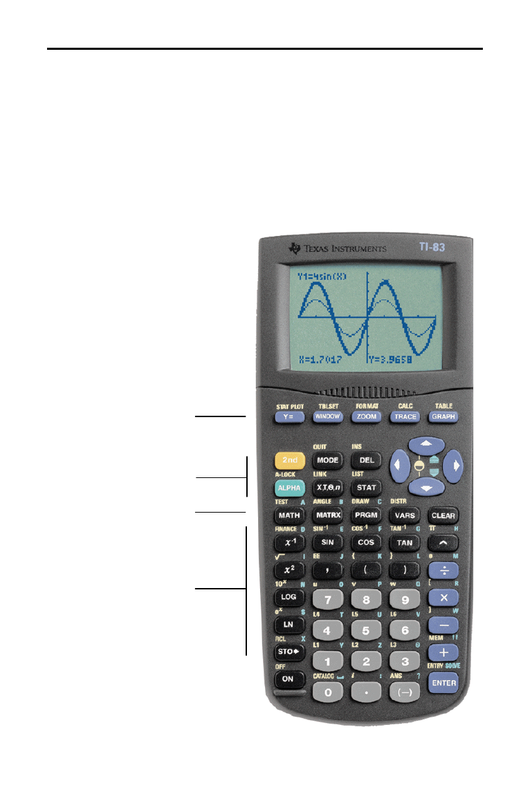
Generally, the keyboard is divided into these zones: graphing keys, editing
keys, advanced function keys, and scientific calculator keys.
Graphing keys access the interactive graphing features.
Editing keys allow you to edit expressions and values.
Advanced function keys display menus that access the
advanced functions.
Scientific calculator keys access the capabilities of a
standard scientific calculator.
TI-83 Keyboard
Keyboard Zones
Editing Keys
Advanced
Function Keys
Scientific
Calculator Keys
Graphing Keys
Getting Started 3
8300GETM.DOC TI-83 international English Bob Fedorisko Revised: 02/19/01 11:06 AM Printed: 02/19/01 11:06
AM Page 3 of 18
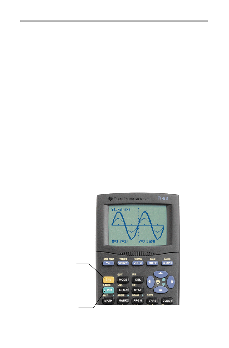
The keys on the TI
.
83 are color-coded to help you easily
locate the key you need.
The gray keys are the number keys. The blue keys along the
right side of the keyboard are the common math functions.
The blue keys across the top set up and display graphs.
The primary function of each key is printed in white on the
key. For example, when you press
, the
MATH
menu is
displayed.
The secondary function of each key is printed in yellow
above the key. When you press the yellow
y
key, the
character, abbreviation, or word printed in yellow above
the other keys becomes active for the next keystroke. For
example, when you press
y
and then
, the
TEST
menu is displayed. This guidebook describes this keystroke
combination as
y
[
TEST
].
The alpha function of each key is printed in green above
the key. When you press the green
ƒ
key, the alpha
character printed in green above the other keys becomes
active for the next keystroke. For example, when you press
ƒ
and then
, the letter
A is entered. This
guidebook describes this keystroke combination as
ƒ
[
A
].
Using the
Color-Coded
Keyboard
Using the
y
and
ƒ
Keys
The
y
key accesses
the second function
printed in yellow above
each key.
The
ƒ
key
accesses the alpha
function printed in
green above each key.
4 Getting Started
8300GETM.DOC TI-83 international English Bob Fedorisko Revised: 02/19/01 11:11 AM Printed: 02/19/01 11:15
AM Page 4 of 18
Displaying a Menu
While using your TI
.
83, you often will need
to access items from its menus.
When you press a key that displays a menu,
that menu temporarily replaces the screen
where you are working. For example, when
you press
, the
MATH
menu is displayed
as a full screen.
A
fter you select an item from a menu, the
screen where you are working usually is
displayed again.
Moving from One Menu to Another
Some keys access more than one menu. When
you press such a key, the names of all
accessible menus are displayed on the top
line. When you highlight a menu name, the
items in that menu are displayed. Press
~
and
|
to highlight each menu name.
Selecting an Item from a Menu
The number or letter next to the current menu
item is highlighted. If the menu continues
beyond the screen, a down arrow (
$
)
replaces the colon (
:
) in the last displayed
item. If you scroll beyond the last displayed
item, an up arrow (
#
) replaces the colon in
the first item displayed.You can select an item
in either of two ways.
¦
Press
†
or
}
to move the cursor to the
number or letter of the item; press
Í
.
¦
Press the key or key combination for the
number or letter next to the item.
Leaving a Menu without Making a Selection
You can leave a menu without making a
selection in any of three ways.
¦
Press
‘
to return to the screen
where you were.
¦
Press
y
[
QUIT
] to return to the home
screen.
¦
Press a key for another menu or screen.
TI-83 Menus
Getting Started 5
8300GETM.DOC TI-83 international English Bob Fedorisko Revised: 02/19/01 11:06 AM Printed: 02/19/01 11:06
AM Page 5 of 18
Before starting the sample problems in this chapter, follow the steps on this
page to reset the TI
.
83 to its factory settings and clear all memory. This
ensures that the keystrokes in this chapter will produce the illustrated results.
To reset the TI
.
83, follow these steps.
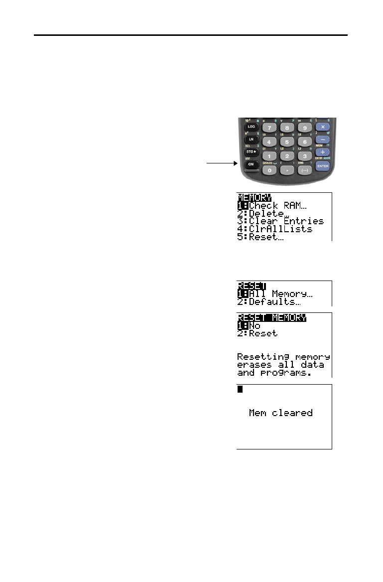
1. Press
É
to turn on the calculator.
2. Press and release
y
, and then press
[
MEM
] (above
Ã
).
When you press
y
, you access the
operation printed in yellow above the next
key that you press. [
MEM
] is the
y
operation of the
Ã
key.
The
MEMORY
menu is displayed.
3. Press 5 to select 5:Reset.
The
RESET
menu is displayed.
4. Press 1 to select 1:All Memory.
The
RESET MEMORY
menu is displayed.
5. Press 2 to select 2:Reset.
All memory is cleared, and the calculator
is reset to the factory default settings.
When you reset the TI
.
83, the display
contrast is reset.
¦
If the screen is very light or blank, press
and release
y
, and then press and
hold
}
to darken the screen.
¦
If the screen is very dark, press and
release
y
, and then press and hold
†
to lighten the screen.
First Steps
6 Getting Started
8300GETM.DOC TI-83 international English Bob Fedorisko Revised: 02/19/01 11:06 AM Printed: 02/19/01 11:06
AM Page 6 of 18
Use the quadratic formula to solve the quadratic equations 3X
2
+ 5X + 2 = 0
and 2X
2
N
X + 3 = 0. Begin with the equation 3X
2
+ 5X + 2 = 0.
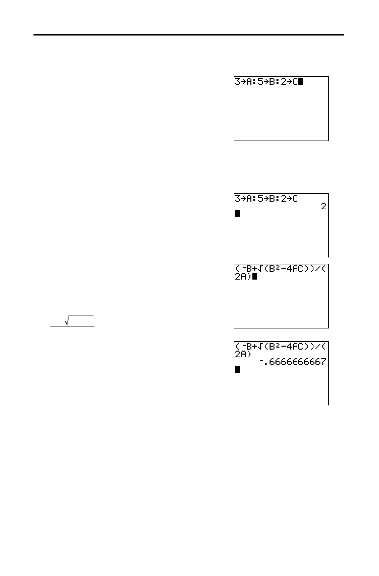
1. Press
3
¿
ƒ
[
A
] (above
) to
store the coefficient of the X
2
term.
2. Press
ƒ
[
:
] (above
Ë
). The colon
allows you to enter more than one
instruction on a line.
3. Press
5
¿
ƒ
[
B
] (above
) to
store the coefficient of the X
term. Press
ƒ
[
:
] to enter a new instruction on
the same line. Press
2
¿
ƒ
[
C
]
(above
) to store the constant.
4. Press
Í
to store the values to the
variables A, B, and C.
The last value you stored is shown on the
right side of the display. The cursor moves
to the next line, ready for your next entry.
5. Press
£
Ì
ƒ
[
B
]
Ã
y
[
‡
]
ƒ
[
B
]
¡
¹
4
ƒ
[
A
]
ƒ
[
C
]
¤
¤
¥
£
2
ƒ
[
A
]
¤
to enter the expression for
one of the solutions for the quadratic
formula,
−
+−
bb ac
a
2
4
2
6. Press
Í
to find one solution for the
equation 3X
2
+ 5X + 2 = 0.
The answer is shown on the right side of
the display. The cursor moves to the next
line, ready for you to enter the next
expression.
Entering a Calculation: The Quadratic Formula
Getting Started 7
8300GETM.DOC TI-83 international English Bob Fedorisko Revised: 02/19/01 11:06 AM Printed: 02/19/01 11:06
AM Page 7 of 18
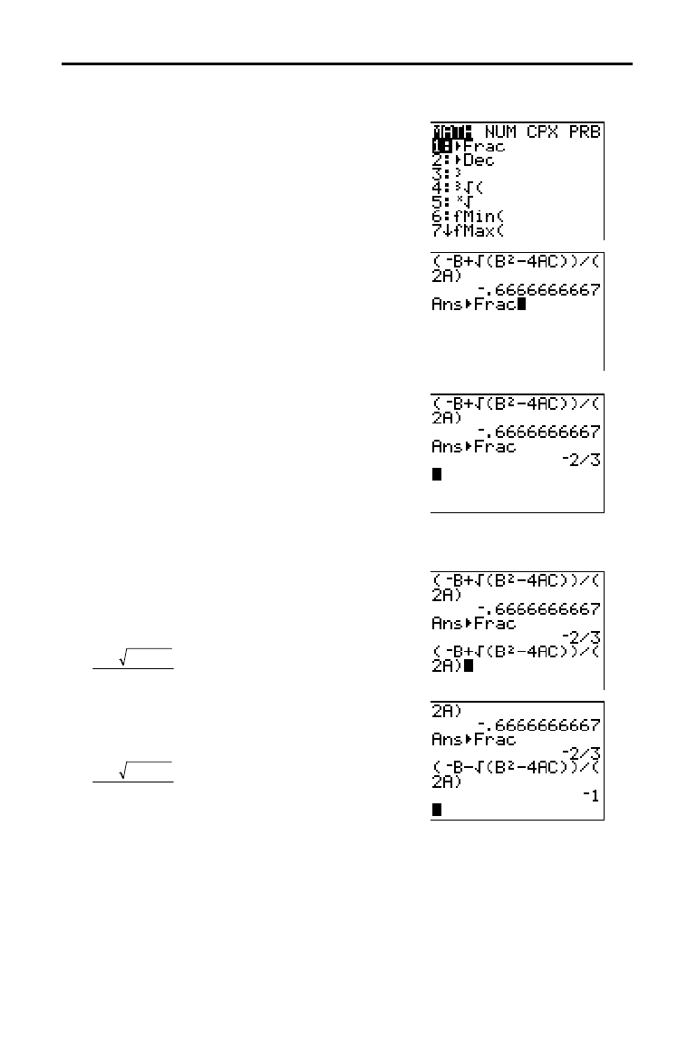
You can show the solution as a fraction.
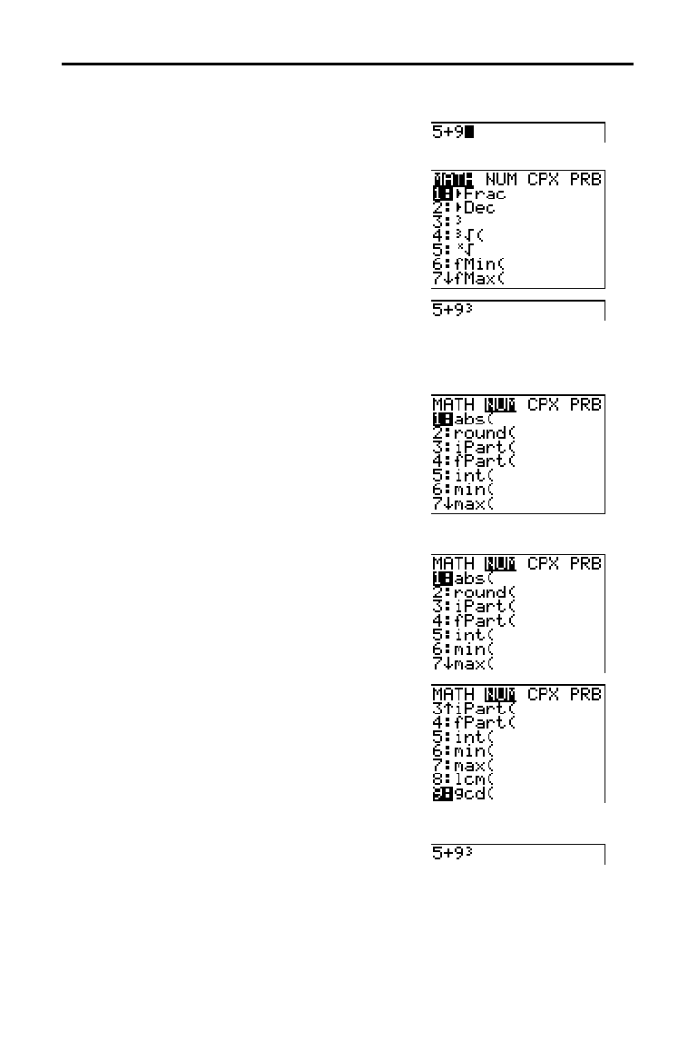
1. Press
to display the
MATH
menu.
2. Press 1 to select 1:
4
Frac from the
MATH
menu.
When you press
1, Ans
4
Frac is displayed on
the home screen.
Ans is a variable that
contains the last calculated answer.
3. Press
Í
to convert the result to a
fraction.
To save keystrokes, you can recall the last expression you entered, and then
edit it for a new calculation.
4. Press
y
[
ENTRY
] (above
Í
) to recall
the fraction conversion entry, and then
press
y
[
ENTRY
] again to recall the
quadratic-formula expression,
−
+−
bb ac
a
2
4
2
5. Press
}
to move the cursor onto the + sign
in the formula. Press
¹
to edit the
quadratic-formula expression to become:
−
−−
bb ac
a
2
4
2
6. Press
Í
to find the other solution for
the quadratic equation 3X
2
+ 5X + 2 = 0.
Converting to a Fraction: The Quadratic Formula
8 Getting Started
8300GETM.DOC TI-83 international English Bob Fedorisko Revised: 02/19/01 11:06 AM Printed: 02/19/01 11:06
AM Page 8 of 18
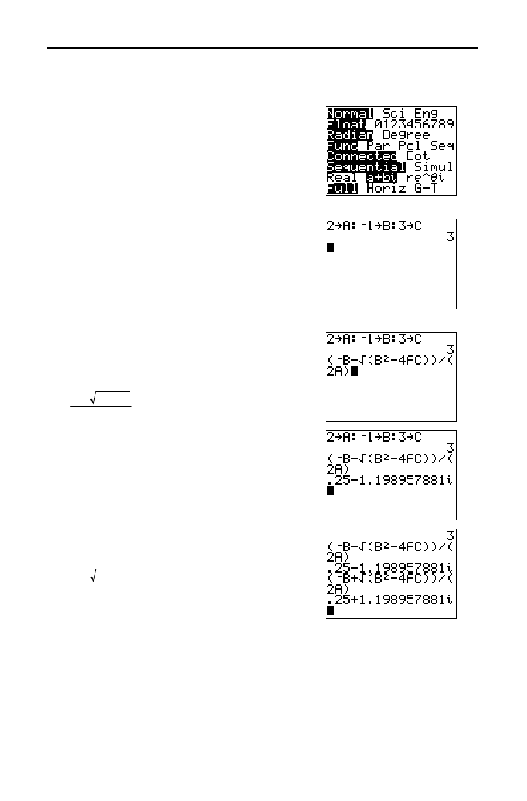
Now solve the equation 2X
2
N
X + 3 = 0. When you set a+b
i
complex number
mode, the TI
.
83 displays complex results.
1. Press
z
†
†
†
†
†
†
(6 times), and
then press
~
to position the cursor over
a+b
i
. Press
Í
to select
a+b
i
complex-
number mode.
2. Press
y
[
QUIT
] (above
z
) to return to
the home screen, and then press
‘
to
clear it.
3. Press 2
¿
ƒ
[
A
]
ƒ
[
:
]
Ì
1
¿
ƒ
[
B
]
ƒ
[
:
] 3
¿
ƒ
[
C
]
Í
.
The coefficient of the X
2
term, the
coefficient of the X term, and the constant
for the new equation are stored to A, B,
and C, respectively.
4. Press
y
[
ENTRY
] to recall the store
instruction, and then press
y
[
ENTRY
]
again to recall the quadratic-formula
expression,
−
−−
bb ac
a
2
4
2
5. Press
Í
to find one solution for the
equation 2X
2
N
X + 3 = 0.
6. Press
y
[
ENTRY
] repeatedly until this
quadratic-formula expression is displayed:
−
+−
bb ac
a
2
4
2
7. Press
Í
to find the other solution for
the quadratic equation: 2X
2
N
X + 3 = 0.
Note:
An alternative for solving equations for real numbers is to use the built-in Equation
Solver (Chapter 2).
Displaying Complex Results: The Quadratic Formula
Getting Started 9
8300GETM.DOC TI-83 international English Bob Fedorisko Revised: 02/19/01 11:06 AM Printed: 02/19/01 11:06
AM Page 9 of 18
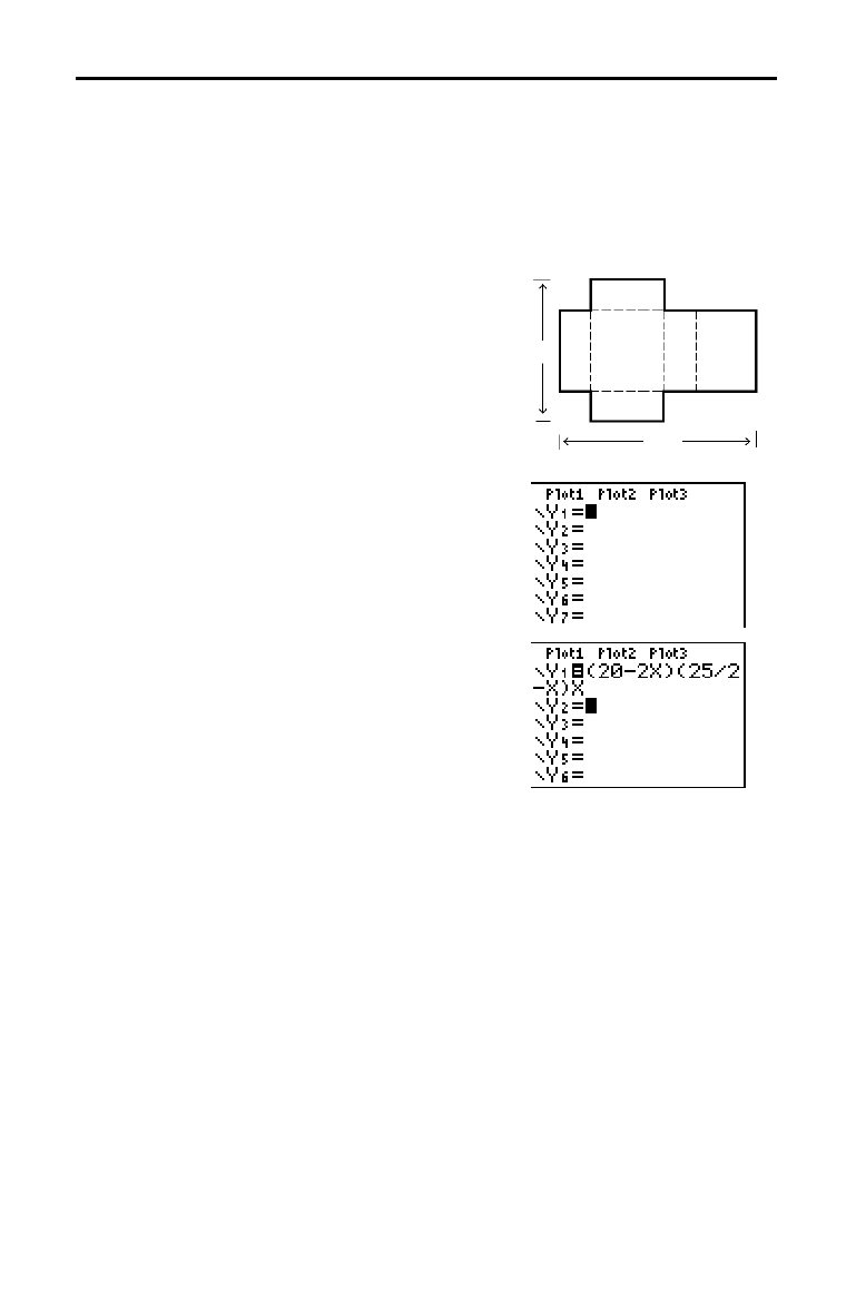
Take a 20 cm. × 25 cm. sheet of paper and cut X × X squares from two corners.
Cut X × 12.5 cm. rectangles from the other two corners as shown in the
diagram below. Fold the paper into a box with a lid. What value of X would
give your box the maximum volume V? Use the table and graphs to determine
the solution.
Begin by defining a function that describes the
v
olume of the box.
From the diagram: 2X + A = 20
2X + 2B = 25
V = A B X
Substituting: V = (20
N
2X) (25
à
2
N
X) X
1. Press
o
to display the
Y=
editor, which is
where you define functions for tables and
graphing.
2. Press
£
20
¹
2
„
¤
£
25
¥
2
¹
„
¤
„
Í
to define the
volume function as
Y
1
in terms of X.
„
lets you enter
X quickly, without
having to press
ƒ
. The highlighted
=
sign indicates that Y
1
is selected.
Defining a Function: Box with Lid
20
A
X
X B X B
25
10 Getting Started
8300GETM.DOC TI-83 international English Bob Fedorisko Revised: 02/19/01 11:06 AM Printed: 02/19/01 11:06
AM Page 10 of 18
The table feature of the TI
.
83 displays numeric information about a function.
You can use a table of values from the function defined on page 9 to estimate
an answer to the problem.
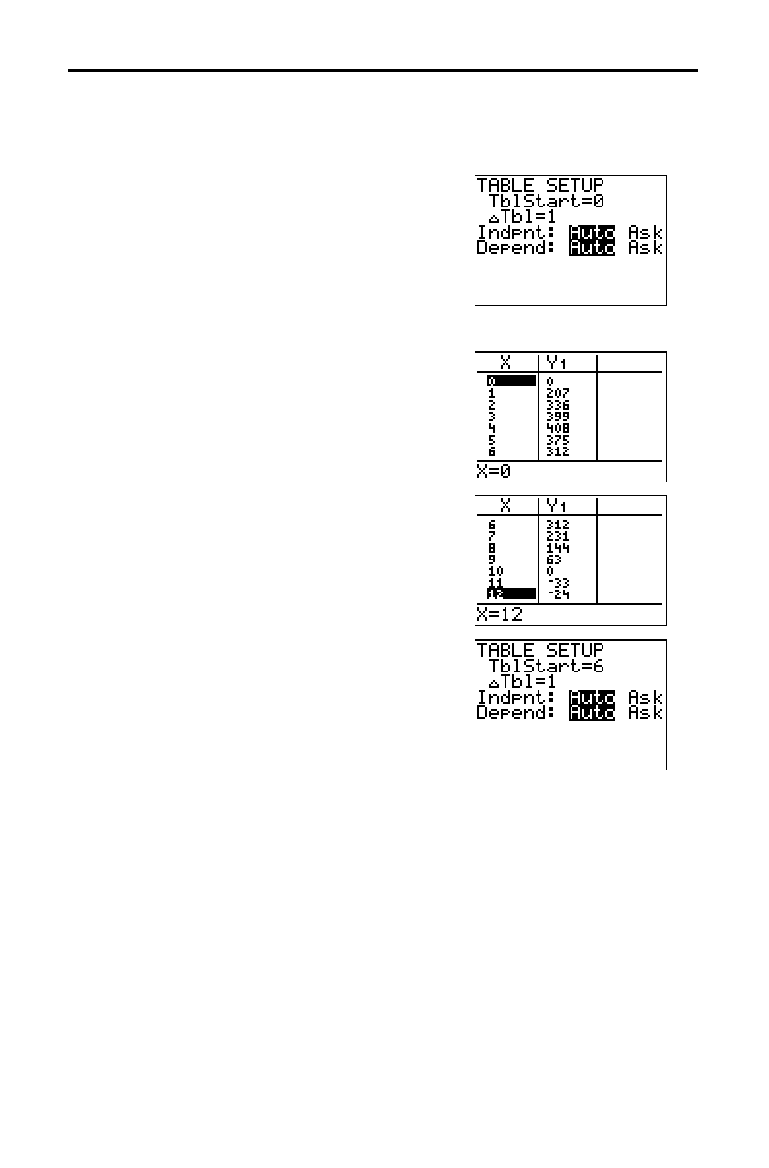
1. Press
y
[
TBLSET
] (above
p
) to
display the
TABLE SETUP
menu.
2. Press
Í
to accept
TblStart=0.
3. Press
1
Í
to define the table increment
@
Tbl=1
. Leave Indpnt: Auto and
Depend: Auto so that the table will be
generated automatically.
4. Press
y
[
TABLE
] (above
s
) to display
the table.
Notice that the maximum value for
Y
1
(box’s volume) occurs when X is about 4,
between
3 and 5.
5. Press and hold
†
to scroll the table until a
negative result for
Y
1
is displayed.
Notice that the maximum length of
X for
this problem occurs where the sign of
Y
1
(box’s volume) changes from positive to
negative, between
10 and 11.
6. Press
y
[
TBLSET
].
Notice that
TblStart has changed to 6 to
reflect the first line of the table as it was
last displayed. (In step 5, the first value of
X displayed in the table is 6.)
Defining a Table of Values: Box with Lid
Getting Started 11
8300GETM.DOC TI-83 international English Bob Fedorisko Revised: 02/19/01 11:06 AM Printed: 02/19/01 11:06
AM Page 11 of 18
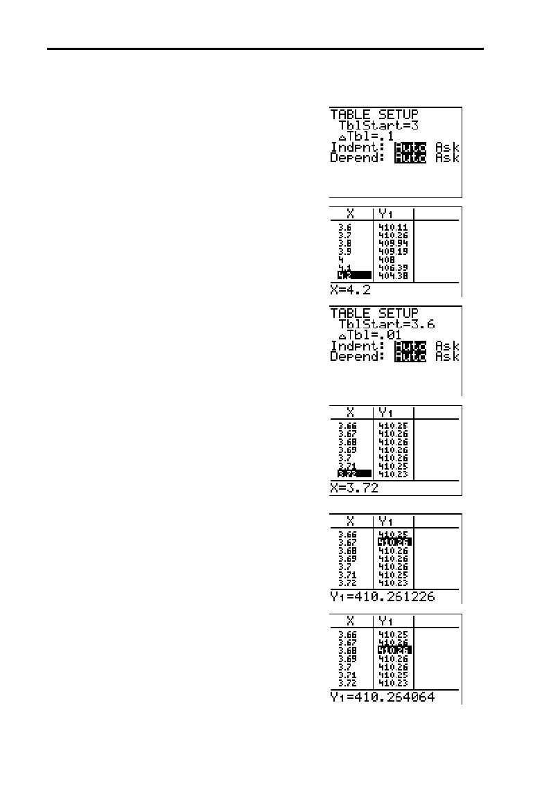
You can adjust the way a table is displayed to get more information about a
defined function. With smaller values for
@
Tbl
, you can zoom in on the table.
1. Press
3
Í
to set TblStart. Press
Ë
1
Í
to set
@
Tbl
.
This adjusts the table setup to get a more
accurate estimate of
X for maximum
volume
Y
1
.
2. Press
y
[
TABLE
].
3. Press
†
and
}
to scroll the table.
Notice that the maximum value for
Y
1
is
410.26, which occurs at X=3.7. Therefore,
the maximum occurs where
3.6<X<3.8.
4. Press
y
[
TBLSET
]. Press 3
Ë
6
Í
to
set
TblStart. Press
Ë
01
Í
to set
@
Tbl
.
5. Press
y
[
TABLE
], and then press
†
and
}
to scroll the table.
Four equivalent maximum values are
shown,
410.60 at X=3.67, 3.68, 3.69, and
3.70.
6. Press
†
and
}
to move the cursor to 3.67.
Press
~
to move the cursor into the
Y
1
column.
The value of
Y
1
at X=3.67 is displayed on
the bottom line in full precision as
410.261226.
7. Press
†
to display the other maximums.
The value of
Y
1
at X=3.68 in full precision is
410.264064, at X=3.69 is 410.262318, and at
X=3.7 is 410.256.
The maximum volume of the box would
occur at
3.68 if you could measure and cut
the paper at .01-cm. increments.
Zooming In on the Table: Box with Lid
12 Getting Started
8300GETM.DOC TI-83 international English Bob Fedorisko Revised: 02/19/01 11:06 AM Printed: 02/19/01 11:06
AM Page 12 of 18
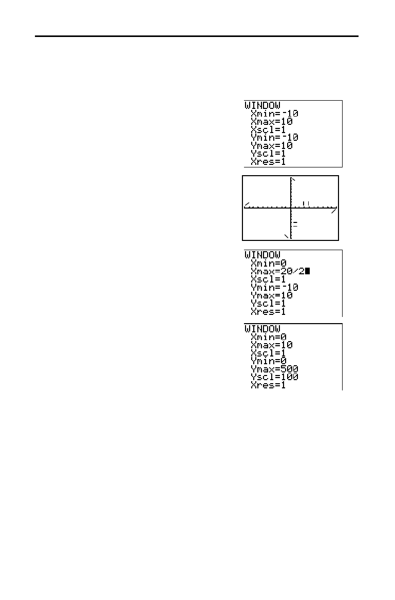
You also can use the graphing features of the TI
.
83 to find the maximum value
of a previously defined function. When the graph is activated, the viewing
window defines the displayed portion of the coordinate plane. The values of
the window variables determine the size of the viewing window.
1. Press
p
to display the window
editor, where you can view and edit the
values of the window variables.
The standard window variables define the
viewing window as shown.
Xmin, Xmax,
Ymin, and Ymax define the boundaries of
the display.
Xscl and Yscl define the
distance between tick marks on the
X and
Y axes. Xres controls resolution.
Xmax
Ymin
Ymax
Xscl
Yscl
Xmin
2. Press 0
Í
to define Xmin.
3. Press
20
¥
2 to define Xmax using an
expression.
4. Press
Í
. The expression is evaluated,
and
10 is stored in Xmax. Press
Í
to
accept
Xscl as 1.
5. Press
0
Í
500
Í
100
Í
1
Í
to define the remaining window variables.
Setting the Viewing Window: Box with Lid
Getting Started 13
8300GETM.DOC TI-83 international English Bob Fedorisko Revised: 02/19/01 11:06 AM Printed: 02/19/01 11:06
AM Page 13 of 18
Now that you have defined the function to be graphed and the window in
which to graph it, you can display and explore the graph. You can trace along a
function using the
TRACE
feature.
1. Press
s
to graph the selected function
in the viewing window.
The graph of
Y
1
=(20
N
2X)(25
à
2
N
X)X is
displayed.
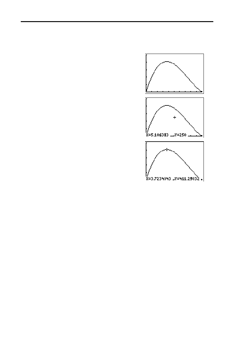
2. Press
~
to activate the free-moving graph
cursor.
The
X and Y coordinate values for the
position of the graph cursor are displayed
on the bottom line.
3. Press
|
,
~
,
}
, and
†
to move the free-
moving cursor to the apparent maximum
of the function.
As you move the cursor, the
X and Y
coordinate values are updated continually.
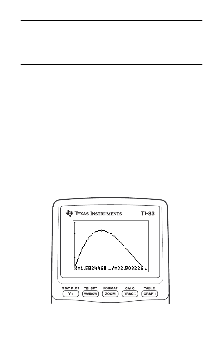
Displaying and Tracing the Graph: Box with Lid
14 Getting Started
8300GETM.DOC TI-83 international English Bob Fedorisko Revised: 02/19/01 11:06 AM Printed: 02/19/01 11:06
AM Page 14 of 18
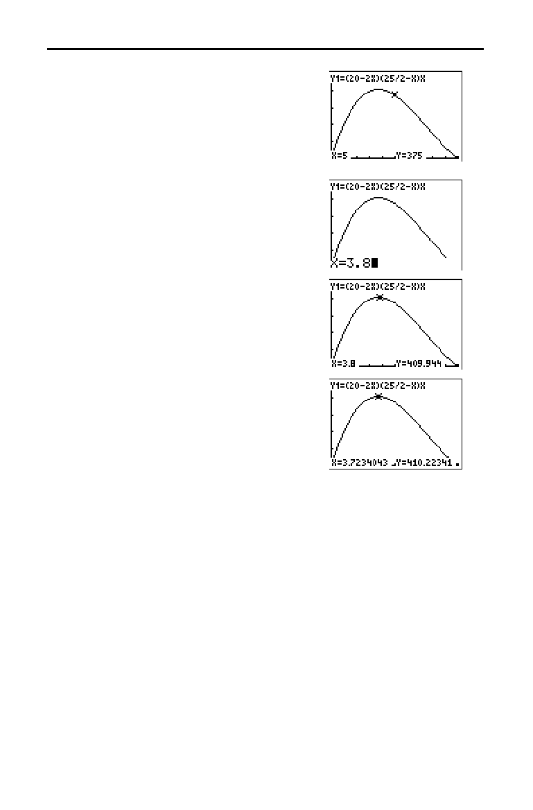
4. Press
r
. The trace cursor is displayed
on the
Y
1
function.
The function that you are tracing is
displayed in the top-left corner.
5. Press
|
and
~
to trace along
Y
1
, one X dot
at a time, evaluating
Y
1
at each X.
You also can enter your estimate for the
maximum value of
X.
6. Press
3
Ë
8. When you press a number key
while in
TRACE
, the X= prompt is displayed
in the bottom-left corner.
7. Press
Í
.
The trace cursor jumps to the point on the
Y
1
function evaluated at X=3.8.
8. Press
|
and
~
until you are on the
maximum
Y value.
This is the maximum of
Y
1
(X) for the X
pixel values. The actual, precise maximum
may lie between pixel values.
Getting Started 15
8300GETM.DOC TI-83 international English Bob Fedorisko Revised: 02/19/01 11:06 AM Printed: 02/19/01 11:06
AM Page 15 of 18
To help identify maximums, minimums, roots, and intersections of functions,
you can magnify the viewing window at a specific location using the
ZOOM
instructions.
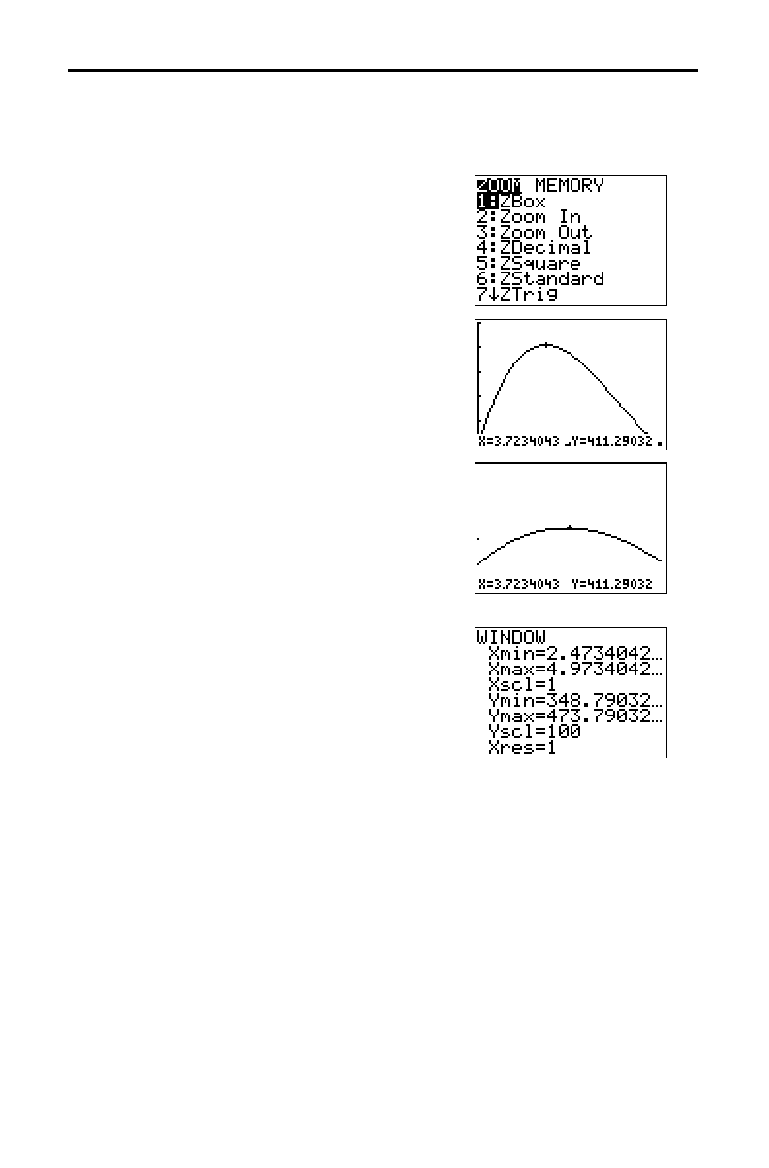
1. Press
q
to display the
ZOOM
menu.
This menu is a typical TI
.
83 menu. To
select an item, you can either press the
number or letter next to the item, or you
can press
†
until the item number or letter
is highlighted, and then press
Í
.
2. Press 2 to select 2:Zoom In.
The graph is displayed again. The cursor
has changed to indicate that you are using
a
ZOOM
instruction.
3. With the cursor near the maximum value
of the function (as in step 8 on page 14),
press
Í
.
The new viewing window is displayed.
Both
Xmax
N
Xmin and Ymax
N
Ymin have
been adjusted by factors of 4, the default
values for the zoom factors.
4. Press
p
to display the new window
settings.
Zooming In on the Graph: Box with Lid
16 Getting Started
8300GETM.DOC TI-83 international English Bob Fedorisko Revised: 02/19/01 11:06 AM Printed: 02/19/01 11:06
AM Page 16 of 18
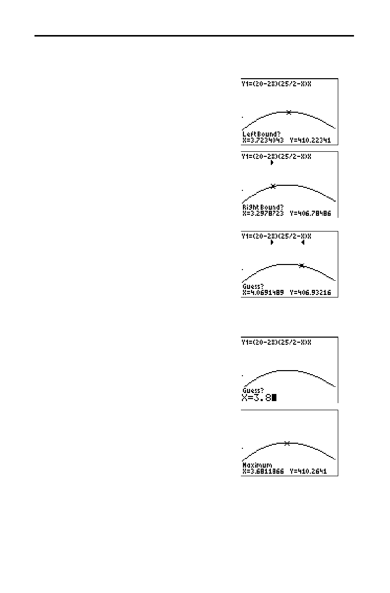
You can use a
CALCULATE
menu operation to calculate a local maximum of a
function.
1. Press
y
[
CALC
] (above
r
) to display
the
CALCULATE
menu. Press 4 to select
4:maximum.
The graph is displayed again with a
Left Bound? prompt.
2. Press
|
to trace along the curve to a point
to the left of the maximum, and then press
Í
.
A
4
at the top of the screen indicates the
selected bound.
A
Right Bound? prompt is displayed.
3. Press
~
to trace along the curve to a point
to the right of the maximum, and then
press
Í
.
A
3
at the top of the screen indicates the
selected bound.
A
Guess? prompt is displayed.
4. Press
|
to trace to a point near the
maximum, and then press
Í
.
Or, press
3
Ë
8, and then press
Í
to
enter a guess for the maximum.
When you press a number key in
TRACE
,
the
X= prompt is displayed in the bottom-
left corner.
Notice how the values for the calculated
maximum compare with the maximums
found with the free-moving cursor, the
trace cursor, and the table.
Note:
In steps 2 and 3 above, you can enter values
directly for Left Bound and Right Bound, in the same
way as described in step 4.
Finding the Calculated Maximum: Box with Lid

Getting Started 17
8300GETM.DOC TI-83 international English Bob Fedorisko Revised: 02/19/01 11:06 AM Printed: 02/19/01 11:06
AM Page 17 of 18
Getting Started has introduced you to basic TI
.
83 operation. This guidebook
describes in detail the features you used in Getting Started. It also covers the
other features and capabilities of the TI
.
83.
You can store, graph, and analyze up to 10 functions
(Chapter 3), up to six parametric functions (Chapter 4), up
to six polar functions (Chapter 5), and up to three
sequences (Chapter 6). You can use
DRAW
operations to
annotate graphs (Chapter 8).
You can generate sequences and graph them over time. Or,
you can graph them as web plots or as phase plots
(Chapter 6).
You can create function evaluation tables to analyze many
functions simultaneously (Chapter 7).
You can split the screen horizontally to display both a
graph and a related editor (such as the
Y=
editor), the
table, the stat list editor, or the home screen. Also, you can
split the screen vertically to display a graph and its table
simultaneously (Chapter 9).
You can enter and save up to 10 matrices and perform
standard matrix operations on them (Chapter 10).
You can enter and save as many lists as memory allows for
use in statistical analyses. You can attach formulas to lists
for automatic computation. You can use lists to evaluate
expressions at multiple values simultaneously and to graph
a family of curves (Chapter 11).
You can perform one- and two-variable, list-based
statistical analyses, including logistic and sine regression
analysis. You can plot the data as a histogram, xyLine,
scatter plot, modified or regular box-and-whisker plot, or
normal probability plot. You can define and store up to
three stat plot definitions (Chapter 12).
Other TI-83 Features
Graphing
Sequences
Tables
Split Screen
Matrices
Lists
Statistics

18 Getting Started
8300GETM.DOC TI-83 international English Bob Fedorisko Revised: 02/19/01 11:06 AM Printed: 02/19/01 11:06
AM Page 18 of 18
You can perform 16 hypothesis tests and confidence
intervals and 15 distribution functions. You can display
hypothesis test results graphically or numerically
(Chapter 13).
You can use time-value-of-money (
TVM
) functions to
analyze financial instruments such as annuities, loans,
mortgages, leases, and savings. You can analyze the value
of money over equal time periods using cash flow
functions. You can amortize loans with the amortization
functions (Chapter 14).
The
CATALOG
is a convenient, alphabetical list of all
functions and instructions on the TI
.
83. You can paste any
function or instruction from the
CATALOG
to the current
cursor location (Chapter 15).
You can enter and store programs that include extensive
control and input/output instructions (Chapter 16).
The TI
.
83 has a port to connect and communicate with
another TI
.
83, a TI
.
82, the Calculator-Based Laboratory
é
(CBL 2
é
, CBL
é
) System, a Calculator-Based Ranger
é
(CBR
é
), or a personal computer. The unit-to-unit link
cable is included with the TI
.
83 (Chapter 19).
Inferential
Statistics
Financial
Functions
CATALOG
Programming
Communication
Link
Operating the TI
-
83 1-1
8301OPER.DOC TI-83 international English Bob Fedorisko Revised: 02/19/01 12:09 PM Printed: 02/19/01 1:34
PM Page 1 of 24
1
Operatin
g
the TI-83
Turning On and Turning Off the TI
.
83
....................
1-2
Setting the Display Contrast
.............................
1-3
The Display
..............................................
1-4
Entering Expressions and Instructions
...................
1-6
TI
.
83 Edit Keys
..........................................
1-8
Setting Modes
...........................................
1-9
Using TI
.
83 Variable Names
.............................
1-13
Storing Variable Values
..................................
1-14
Recalling Variable Values
................................
1-15
ENTRY
(Last Entry) Storage Area
........................
1-16
Ans
(Last Answer) Storage Area
.........................
1-18
TI
.
83 Menus
.............................................
1-19
VARS
and
VARS Y
.
VARS
Menus
.........................
1-21
Equation Operating System (EOS
é
)
.....................
1-22
Error Conditions
.........................................
1-24
Contents

1-2 Operating the TI
-
83
8301OPER.DOC TI-83 international English Bob Fedorisko Revised: 02/19/01 12:09 PM Printed: 02/19/01 1:34
PM Page 2 of 24
To turn on the TI
.
83, press
É
.
•
If you previously had turned off the calculator by
pressing
y
[
OFF
], the TI
.
83 displays the home screen
as it was when you last used it and clears any error.
•
If Automatic Power Down™ (APD
é
) had previously
turned off the calculator, the TI
.
83 will return exactly as
you left it, including the display, cursor, and any error.
To prolong the life of the batteries, APD turns off the TI
.
83
automatically after about five minutes without any activity.
To turn off the TI
.
83 manually, press
y
[
OFF
].
•
All settings and memory contents are retained by
Constant Memory
é
.
•
Any error condition is cleared.
The TI
.
83 uses four AAA alkaline batteries and has a user-
replaceable backup lithium battery (CR1616 or CR1620).
To replace batteries without losing any information stored
in memory, follow the steps in Appendix B.
Turning On and Turning Off the TI-83
Turning On the
Calculator
Turning Off the
Calculator
Batteries
Operating the TI
-
83 1-3
8301OPER.DOC TI-83 international English Bob Fedorisko Revised: 02/19/01 12:09 PM Printed: 02/19/01 1:34
PM Page 3 of 24
You can adjust the display contrast to suit your viewing
angle and lighting conditions. As you change the contrast
setting, a number from
0 (lightest) to 9 (darkest) in the
top-right corner indicates the current level. You may not be
able to see the number if contrast is too light or too dark.
Note:
The TI
.
83 has 40 contrast settings, so each number
0
through
9
represents four settings.
The TI
.
83 retains the contrast setting in memory when it is
turned off.
To adjust the contrast, follow these steps.
1. Press and release the
y
key.
2. Press and hold
†
or
}
, which are below and above the
contrast symbol (yellow, half-shaded circle).
•
†
lightens the screen.
•
}
darkens the screen.
Note:
If you adjust the contrast setting to
0
, the display may become
completely blank. To restore the screen, press and release
y
, and
then press and hold
}
until the display reappears.
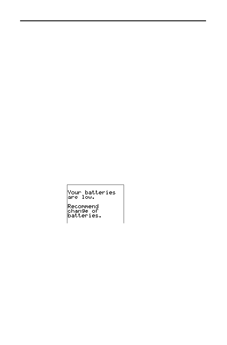
When the batteries are low, a low-battery message is
displayed when you turn on the calculator.
To replace the batteries without losing any information in
memory, follow the steps in Appendix B.
Generally, the calculator will continue to operate for one
or two weeks after the low-battery message is first
displayed. After this period, the TI
.
83 will turn off
automatically and the unit will not operate. Batteries must
be replaced. All memory is retained.
Note:
The operating period following the first low-battery message
could be longer than two weeks if you use the calculator infrequently.
Setting the Display Contrast
Adjusting the
Display Contrast
When to Replace
Batteries
1-4 Operating the TI
-
83
8301OPER.DOC TI-83 international English Bob Fedorisko Revised: 02/19/01 12:09 PM Printed: 02/19/01 1:34
PM Page 4 of 24
The TI
.
83 displays both text and graphs. Chapter 3
describes graphs. Chapter 9 describes how the TI
.
83 can
display a horizontally or vertically split screen to show
graphs and text simultaneously.
The home screen is the primary screen of the TI
.
83. On
this screen, enter instructions to execute and expressions
to evaluate. The answers are displayed on the same screen.
When text is displayed, the TI
.
83 screen can display a
maximum of eight lines with a maximum of 16 characters
per line. If all lines of the display are full, text scrolls off
the top of the display. If an expression on the home screen,
the
Y=
editor (Chapter 3), or the program editor
(Chapter 16) is longer than one line, it wraps to the
beginning of the next line. In numeric editors such as the
window screen (Chapter 3), a long expression scrolls to
the right and left.
When an entry is executed on the home screen, the answer
is displayed on the right side of the next line.
Entry
Answer
The mode settings control the way the TI
.
83 interprets
expressions and displays answers (page 1
.
9).
If an answer, such as a list or matrix, is too long to display
entirely on one line, an ellipsis (
...) is displayed to the right
or left. Press
~
and
|
to scroll the answer.
Entry
Answer
To return to the home screen from any other screen, press
y
[
QUIT
].
When the TI
.
83 is calculating or graphing, a vertical
moving line is displayed as a busy indicator in the top-right
corner of the screen. When you pause a graph or a
program, the busy indicator becomes a vertical moving
dotted line.
The Display
Types of
Displays
Home Screen
Displaying
Entries and
Answers
Returning to the
Home Screen
Busy Indicator

Operating the TI
-
83 1-5
8301OPER.DOC TI-83 international English Bob Fedorisko Revised: 02/19/01 12:09 PM Printed: 02/19/01 1:34
PM Page 5 of 24
In most cases, the appearance of the cursor indicates what
will happen when you press the next key or select the next
menu item to be pasted as a character.
Cursor Appearance Effect of Next Keystroke
Entry Solid rectan
g
le
$
A character is entered at the
cursor; any existin
g
character is
overwritten
Insert Underline
__
A character is inserted in front of
the cursor location
Second Reverse arrow
Þ
A 2nd character
(
yellow on the
keyboard
)
is entered or a 2nd
operation is executed
A
lpha Reverse A
Ø
An alpha character
(g
reen on the
keyboard
)
is entered or
SOLVE
is
executed
Full Checkerboard
rectan
g
le
#
No entry; the maximum characters
are entered at a prompt or memory
is full
If you press
ƒ
during an insertion, the cursor becomes
an underlined
A
(
A
) If you press
y
during an insertion, the
underline cursor becomes an underlined
#
(
#
).
Graphs and editors sometimes display additional cursors,
which are described in other chapters.
Display Cursors

1-6 Operating the TI
-
83
8301OPER.DOC TI-83 international English Bob Fedorisko Revised: 02/19/01 12:09 PM Printed: 02/19/01 1:34
PM Page 6 of 24
An expression is a group of numbers, variables, functions
and their arguments, or a combination of these elements.
An expression evaluates to a single answer. On the TI
.
83,
you enter an expression in the same order as you would
write it on paper. For example,
p
R
2
is an expression.
You can use an expression on the home screen to calculate
an answer. In most places where a value is required, you
can use an expression to enter a value.
To create an expression, you enter numbers, variables, and
functions from the keyboard and menus. An expression is
completed when you press
Í
, regardless of the cursor
location. The entire expression is evaluated according to
Equation Operating System (EOS
é
) rules (page 1
.
22), and
the answer is displayed.
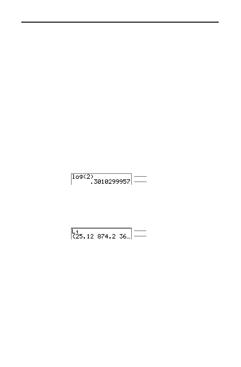
Most TI
.
83 functions and operations are symbols
comprising several characters. You must enter the symbol
from the keyboard or a menu; do not spell it out. For
example, to calculate the log of 45, you must press
«
45.
Do not enter the letters
L, O, and G. If you enter LOG, the
TI
.
83 interprets the entry as implied multiplication of the
variables
L, O, and G.
Calculate 3.76 ÷ (
L
7.9 +
‡
5) + 2 log 45.
3
Ë
76
¥
£
Ì
7
Ë
9
Ã
y
[
‡
] 5
¤
¤
Ã
2
«
45
¤
Í
To enter two or more expressions or instructions on a line,
separate them with colons (
ƒ
[
:
]). All instructions are
stored together in last entry (
ENTRY
; page 1
.
16).
Entering Expressions and Instructions
What Is an
Expression?
Entering an
Expression
Multiple Entries
on a Line
Operating the TI
-
83 1-7
8301OPER.DOC TI-83 international English Bob Fedorisko Revised: 02/19/01 12:09 PM Printed: 02/19/01 1:34
PM Page 7 of 24
To enter a number in scientific notation, follow these
steps.
1. Enter the part of the number that precedes the
exponent. This value can be an expression.
2. Press
y
[
EE
].
å
is pasted to the cursor location.
3. If the exponent is negative, press
Ì
, and then enter the
exponent, which can be one or two digits.
When you enter a number in scientific notation, the TI
.
83
does not automatically display answers in scientific or
engineering notation. The mode settings (page 1
.
9) and the
size of the number determine the display format.
A function returns a value. For example,
÷,
L
, +,
‡
(
, and log(
are the functions in the example on page 1
.
6. In general, the
first letter of each function is lowercase on the TI
.
83. Most
functions take at least one argument, as indicated by an open
parenthesis (
( ) following the name. For example, sin(
requires one argument, sin(
value
).
An instruction initiates an action. For example,
ClrDraw is
an instruction that clears any drawn elements from a
graph. Instructions cannot be used in expressions. In
general, the first letter of each instruction name is
uppercase. Some instructions take more than one
argument, as indicated by an open parenthesis (
( ) at the
end of the name. For example,
Circle( requires three
arguments,
Circle(
X
,
Y
,
radius
).
To interrupt a calculation or graph in progress, which
would be indicated by the busy indicator, press
É
.
When you interrupt a calculation, the menu is displayed.
•
To return to the home screen, select
1:Quit.
•
To go to the location of the interruption, select
2:Goto.
When you interrupt a graph, a partial graph is displayed.
•
To return to the home screen, press
‘
or any
nongraphing key.
•
To restart graphing, press a graphing key or select a
graphing instruction.
Entering a
Number in
Scientific
Notation
Functions
Instructions
Interrupting a
Calculation

1-8 Operating the TI
-
83
8301OPER.DOC TI-83 international English Bob Fedorisko Revised: 02/19/01 12:09 PM Printed: 02/19/01 1:34
PM Page 8 of 24
Keystrokes Result
~
or
|
Moves the cursor within an expression; these keys repeat.
}
or
†
Moves the cursor from line to line within an expression that
occupies more than one line; these keys repeat.
On the top line of an expression on the home screen,
}
moves
the cursor to the beginning of the expression.
On the bottom line of an expression on the home screen,
†
moves the cursor to the end of the expression.
y
|
Moves the cursor to the beginning of an expression.
y
~
Moves the cursor to the end of an expression.
Í
Evaluates an expression or executes an instruction.
‘
On a line with text on the home screen, clears the current line.
On a blank line on the home screen, clears everythin
g
on the
home screen.
In an editor, clears the expression or value where the cursor is
located; it does not store a zero.
{
Deletes a character at the cursor; this key repeats.
y
[
INS
] Chan
g
es the cursor to
__
; inserts characters in front of the
underline cursor; to end insertion, press
y
[
INS
] or press
|
,
}
,
~
, or
†
.
y
Chan
g
es the cursor to
Þ
; the next keystroke performs a
2nd
operation
(
an operation in yellow above a key and to the left
)
; to
cancel
2nd
, press
y
again.
ƒ
Chan
g
es the cursor to
Ø
; the next keystroke pastes an alpha
character
(
a character in
g
reen above a key and to the ri
g
ht
)
or
executes
SOLVE
(
Chapters 10 and 11
)
; to cancel
ƒ
, press
ƒ
or press
|
,
}
,
~
, or
†
.
y
[
A
.
LOCK
] Chan
g
es the cursor to
Ø
; sets alpha-lock; subsequent keystrokes
(
on an alpha key
)
paste alpha characters; to cancel alpha-lock,
press
ƒ
; name prompts set alpha-lock automatically.
„
Pastes an
X
in
Func
mode, a
T
in
Par
mode, a
q
in
Pol
mode, or an
n
in
Seq
mode with one keystroke.
TI-83 Edit Keys
Operating the TI
-
83 1-9
8301OPER.DOC TI-83 international English Bob Fedorisko Revised: 02/19/01 12:09 PM Printed: 02/19/01 1:34
PM Page 9 of 24
Mode settings control how the TI
.
83 displays and
interprets numbers and graphs. Mode settings are retained
by the Constant Memory feature when the TI
.
83 is turned
off. All numbers, including elements of matrices and lists,
are displayed according to the current mode settings.
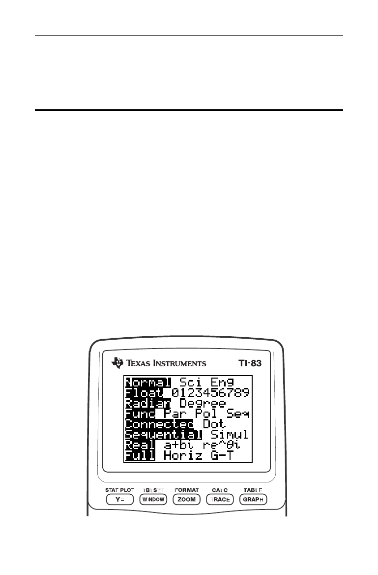
To display the mode settings, press
z
. The current
settings are highlighted. Defaults are highlighted below.
The following pages describe the mode settings in detail.
Normal Sci Eng
Numeric notation
Float 0123456789
Number of decimal places
Radian Degree
Unit of angle measure
Func Par Pol Seq
Type of graphing
Connected Dot
Whether to connect graph points
Sequential Simul
Whether to plot simultaneously
Real a+bi re^
q
i
Real, rectangular cplx, or polar cplx
Full Horiz G-T
Full screen, two split-screen modes
To change mode settings, follow these steps.
1. Press
†
or
}
to move the cursor to the line of the
setting that you want to change.
2. Press
~
or
|
to move the cursor to the setting you
want.
3. Press
Í
.
You can set a mode from a program by entering the name
of the mode as an instruction; for example,
Func or Float.
From a blank command line, select the mode setting from
the mode screen; the instruction is pasted to the cursor
location.
Setting Modes
Checking Mode
Settings
Changing Mode
Settings
Setting a Mode
from a Program

1-10 Operating the TI
-
83
8301OPER.DOC TI-83 international English Bob Fedorisko Revised: 02/19/01 12:09 PM Printed: 02/19/01 1:34
PM Page 10 of 24
Notation modes only affect the way an answer is displayed
on the home screen. Numeric answers can be displayed
with up to 10 digits and a two-digit exponent. You can
enter a number in any format.
Normal notation mode is the usual way we express
numbers, with digits to the left and right of the decimal, as
in
12345.67.
Sci (scientific) notation mode expresses numbers in two
parts. The significant digits display with one digit to the left
of the decimal. The appropriate power of 10 displays to the
right of
E
, as in 1.234567
E
4.
Eng (engineering) notation mode is similar to scientific
notation. However, the number can have one, two, or three
digits before the decimal; and the power-of-10 exponent is
a multiple of three, as in
12.34567
E
3.
Note
: If you select
Normal
notation, but the answer cannot display in
10 digits (or the absolute value is less than .001), the TI
.
83 expresses
the answer in scientific notation.
Float (floating) decimal mode displays up to 10 digits, plus
the sign and decimal.
0123456789 (fixed) decimal mode specifies the number of
digits (
0 through 9) to display to the right of the decimal.
Place the cursor on the desired number of decimal digits,
and then press
Í
.
The decimal setting applies to
Normal, Sci, and Eng
notation modes.
The decimal setting applies to these numbers:
•
An answer displayed on the home screen
•
Coordinates on a graph (Chapters 3, 4, 5, and 6)
•
The
Tangent(
DRAW
instruction equation of the line, x,
and dy/dx values (Chapter 8)
•
Results of
CALCULATE
operations (Chapters 3, 4, 5,
and 6)
•
The regression equation stored after the execution of a
regression model (Chapter 12)
Normal, Sci, Eng
Float,
0123456789

Operating the TI
-
83 1-11
8301OPER.DOC TI-83 international English Bob Fedorisko Revised: 02/19/01 12:09 PM Printed: 02/19/01 1:34
PM Page 11 of 24
Angle modes control how the TI
.
83 interprets angle values
in trigonometric functions and polar/rectangular
conversions.
Radian mode interprets angle values as radians. Answers
display in radians.
Degree mode interprets angle values as degrees. Answers
display in degrees.
Graphing modes define the graphing parameters. Chapters
3, 4, 5, and 6 describe these modes in detail.
Func (function) graphing mode plots functions, where Y is
a function of
X (Chapter 3).
Par (parametric) graphing mode plots relations, where X
and Y are functions of T (Chapter 4).
Pol (polar) graphing mode plots functions, where r is a
function of
q
(Chapter 5).
Seq (sequence) graphing mode plots sequences (Chapter 6).
Connected plotting mode draws a line connecting each
point calculated for the selected functions.
Dot plotting mode plots only the calculated points of the
selected functions.
Radian, Degree
Func, Par, Pol,
Seq
Connected, Dot

1-12 Operating the TI
-
83
8301OPER.DOC TI-83 international English Bob Fedorisko Revised: 02/19/01 12:09 PM Printed: 02/19/01 1:34
PM Page 12 of 24
Sequential graphing-order mode evaluates and plots one
function completely before the next function is evaluated
and plotted.
Simul (simultaneous) graphing-order mode evaluates and
plots all selected functions for a single value of
X and then
evaluates and plots them for the next value of
X.
Note:
Regardless of which graphing mode is selected, the TI
.
83 will
sequentially graph all stat plots before it graphs any functions.
Real mode does not display complex results unless
complex numbers are entered as input.
Two complex modes display complex results.
•
a+b
i
(rectangular complex mode) displays complex
numbers in the form a+b
i
.
•
re^
q
i
(polar complex mode) displays complex numbers
in the form re^
q
i
.
Full screen mode uses the entire screen to display a graph
or edit screen.
Each split-screen mode displays two screens
simultaneously.
•
Horiz (horizontal) mode displays the current graph on
the top half of the screen; it displays the home screen or
an editor on the bottom half (Chapter 9).
•
G
.
T (graph-table) mode displays the current graph on
the left half of the screen; it displays the table screen on
the right half (Chapter 9).
Sequential, Simul
Real, a+b
i
, re^
q
i
Full, Horiz, G
.
T

Operating the TI
-
83 1-13
8301OPER.DOC TI-83 international English Bob Fedorisko Revised: 02/19/01 12:09 PM Printed: 02/19/01 1:34
PM Page 13 of 24
On the TI
.
83 you can enter and use several types of data,
including real and complex numbers, matrices, lists,
functions, stat plots, graph databases, graph pictures, and
strings.
The TI
.
83 uses assigned names for variables and other
items saved in memory. For lists, you also can create your
own five-character names.
Variable Type Names
Real numbers
A
,
B
, . . . ,
Z
,
q
Complex numbers
A
,
B
, . . . ,
Z
,
q
Matrices
ã
A
ä
,
ã
B
ä
,
ã
C
ä
, . . . ,
ã
J
ä
Lists
L
1
,
L
2
,
L
3
,
L
4
,
L
5
,
L
6
, and user-
defined names
Functions
Y
1
,
Y
2
, . . . ,
Y
9
,
Y
0
Parametric equations
X
1T
and
Y
1T
, . . . ,
X
6T
and
Y
6T
Polar functions
r
1
,
r
2
,
r
3
,
r
4
,
r
5
,
r
6
Sequence functions
u
,
v
,
w
Stat plots
Plot1, Plot2, Plot3
Graph databases
GDB1
,
GDB2
, . . . ,
GDB9
,
GDB0
Graph pictures
Pic1
,
Pic2
, . . . ,
Pic9
,
Pic0
Strings
Str1
,
Str2
, . . . ,
Str9
,
Str0
System variables
Xmin
,
Xmax
, and others
•
You can create as many list names as memory will allow
(Chapter 11).
•
Programs have user-defined names and share memory
with variables (Chapter 16).
•
From the home screen or from a program, you can store
to matrices (Chapter 10), lists (Chapter 11), strings
(Chapter 15), system variables such as
Xmax
(Chapter
1),
TblStart
(Chapter 7), and all
Y=
functions (Chapters
3, 4, 5, and 6).
•
From an editor, you can store to matrices, lists, and
Y=
functions (Chapter 3).
•
From the home screen, a program, or an editor, you can
store a value to a matrix element or a list element.
•
You can use
DRAW STO
menu items to store and recall
graph databases and pictures (Chapter 8).
Using TI-83 Variable Names
Variables and
Defined Items
Notes about
Variables
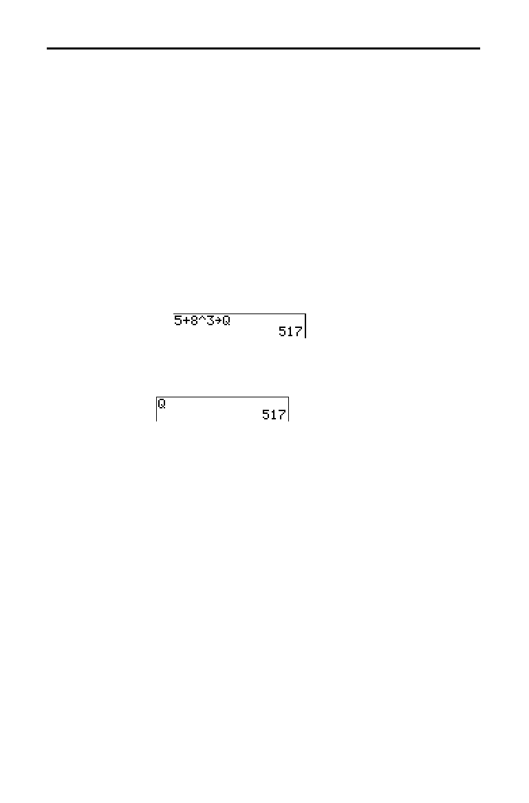
1-14 Operating the TI
-
83
8301OPER.DOC TI-83 international English Bob Fedorisko Revised: 02/19/01 12:09 PM Printed: 02/19/01 1:34
PM Page 14 of 24
Values are stored to and recalled from memory using
variable names. When an expression containing the name
of a variable is evaluated, the value of the variable at that
time is used.
To store a value to a variable from the home screen or a
program using the
¿
key, begin on a blank line and
follow these steps.
1. Enter the value you want to store. The value can be an
expression.
2. Press
¿
.
!
is copied to the cursor location.
3. Press
ƒ
and then the letter of the variable to which
you want to store the value.
4. Press
Í
. If you entered an expression, it is
evaluated. The value is stored to the variable.
To display the value of a variable, enter the name on a
blank line on the home screen, and then press
Í
.
Storing Variable Values
Storing Values in
a Variable
Displaying a
Variable Value
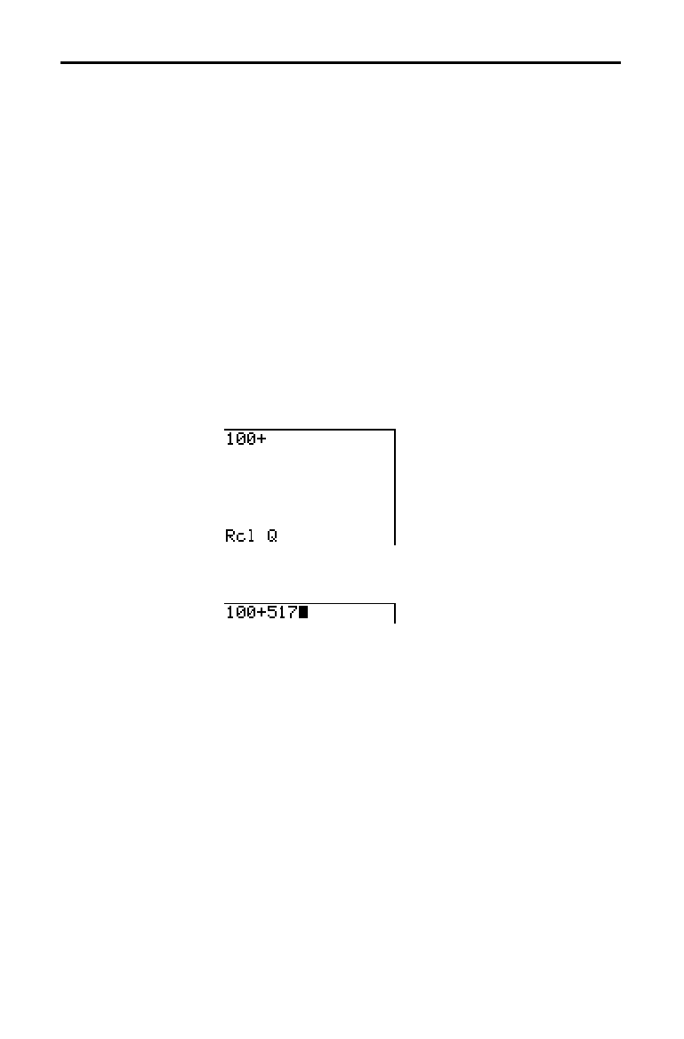
Operating the TI
-
83 1-15
8301OPER.DOC TI-83 international English Bob Fedorisko Revised: 02/19/01 12:09 PM Printed: 02/19/01 1:34
PM Page 15 of 24
To recall and copy variable contents to the current cursor
location, follow these steps. To leave
RCL
, press
‘
.
1. Press
y
ã
RCLä
.
Rcl and the edit cursor are displayed on
the bottom line of the screen.
2. Enter the name of the variable in any of five ways.
•
Press
ƒ
and then the letter of the variable.
•
Press
y
ã
LISTä
, and then select the name of the list,
or press
y
[
Ln
].
•
Press
, and then select the name of the matrix.
•
Press
to display the
VARS
menu or
~
to
display the
VARS Y
.
VARS
menu; then select the type
and then the name of the variable or function.
•
Press
|
, and then select the name of the
program (in the program editor only).
The variable name you selected is displayed on the
bottom line and the cursor disappears.
3. Press
Í
. The variable contents are inserted where
the cursor was located before you began these steps.
Note:
You can edit the characters pasted to the expression without
affecting the value in memory.
Recalling Variable Values
Using Recall
(RCL)
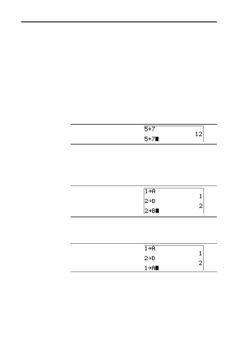
1-16 Operating the TI
-
83
8301OPER.DOC TI-83 international English Bob Fedorisko Revised: 02/19/01 12:09 PM Printed: 02/19/01 1:34
PM Page 16 of 24
When you press
Í
on the home screen to evaluate an
expression or execute an instruction, the expression or
instruction is placed in a storage area called
ENTRY
(last
entry). When you turn off the TI
.
83,
ENTRY
is retained in
memory.
To recall
ENTRY
, press
y
[
ENTRY
]. The last entry is
pasted to the current cursor location, where you can edit
and execute it. On the home screen or in an editor, the
current line is cleared and the last entry is pasted to the
line.
Because the TI
.
83 updates
ENTRY
only when you press
Í
, you can recall the previous entry even if you have
begun to enter the next expression.
5
Ã
7
Í
y
[
ENTRY
]
The TI
.
83 retains as many previous entries as possible in
ENTRY
, up to a capacity of 128 bytes. To scroll those
entries, press
y
[
ENTRY
] repeatedly. If a single entry is
more than 128 bytes, it is retained for
ENTRY
, but it cannot
be placed in the
ENTRY
storage area.
1
¿
ƒ
A
Í
2
¿
ƒ
B
Í
y
[
ENTRY
]
If you press
y
[
ENTRY
] after displaying the oldest stored
entry, the newest stored entry is displayed again, then the
next-newest entry, and so on.
y
[
ENTRY
]
ENTRY (Last Entry) Storage Area
Using ENTRY
(Last Entry)
Accessing a
Previous Entry
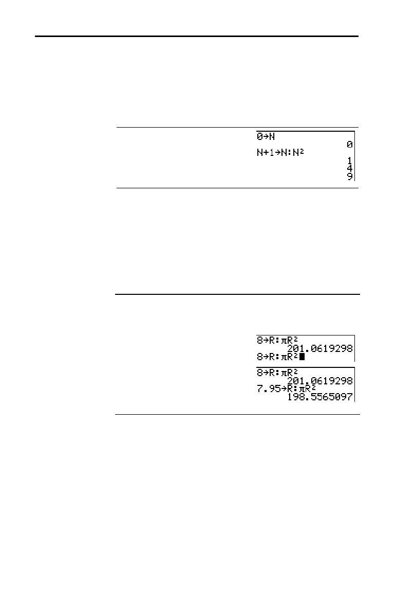
Operating the TI
-
83 1-17
8301OPER.DOC TI-83 international English Bob Fedorisko Revised: 02/19/01 12:09 PM Printed: 02/19/01 1:34
PM Page 17 of 24
After you have pasted the last entry to the home screen
and edited it (if you chose to edit it), you can execute the
entry. To execute the last entry, press
Í
.
To reexecute the displayed entry, press
Í
again. Each
reexecution displays an answer on the right side of the
next line; the entry itself is not redisplayed.
0
¿
ƒ
N
Í
ƒ
N
Ã
1
¿
ƒ
N
ƒ
ã
:
ä
ƒ
N
¡
Í
Í
Í
To store to
ENTRY
two or more expressions or
instructions, separate each expression or instruction with
a colon, then press
Í
. All expressions and instructions
separated by colons are stored in
ENTRY
.
When you press
y
[
ENTRY
], all the expressions and
instructions separated by colons are pasted to the current
cursor location. You can edit any of the entries, and then
execute all of them when you press
Í
.
For the equation A=
p
r
2
, use trial and error to find the radius of a
circle that covers 200 square centimeters. Use 8 as your first
guess.
8
¿
ƒ
R
ƒ
[
:
]
y
[
p
]
ƒ
R
¡
Í
y
[
ENTRY
]
y
|
7
y
[
INS
]
Ë
95
Í
Continue until the answer is as accurate as you want.
Clear Entries (Chapter 18) clears all data that the TI
.
83 is
holding in the
ENTRY
storage area.
Reexecuting the
Previous Entry
Multiple Entry
Values on a Line
Clearing ENTRY
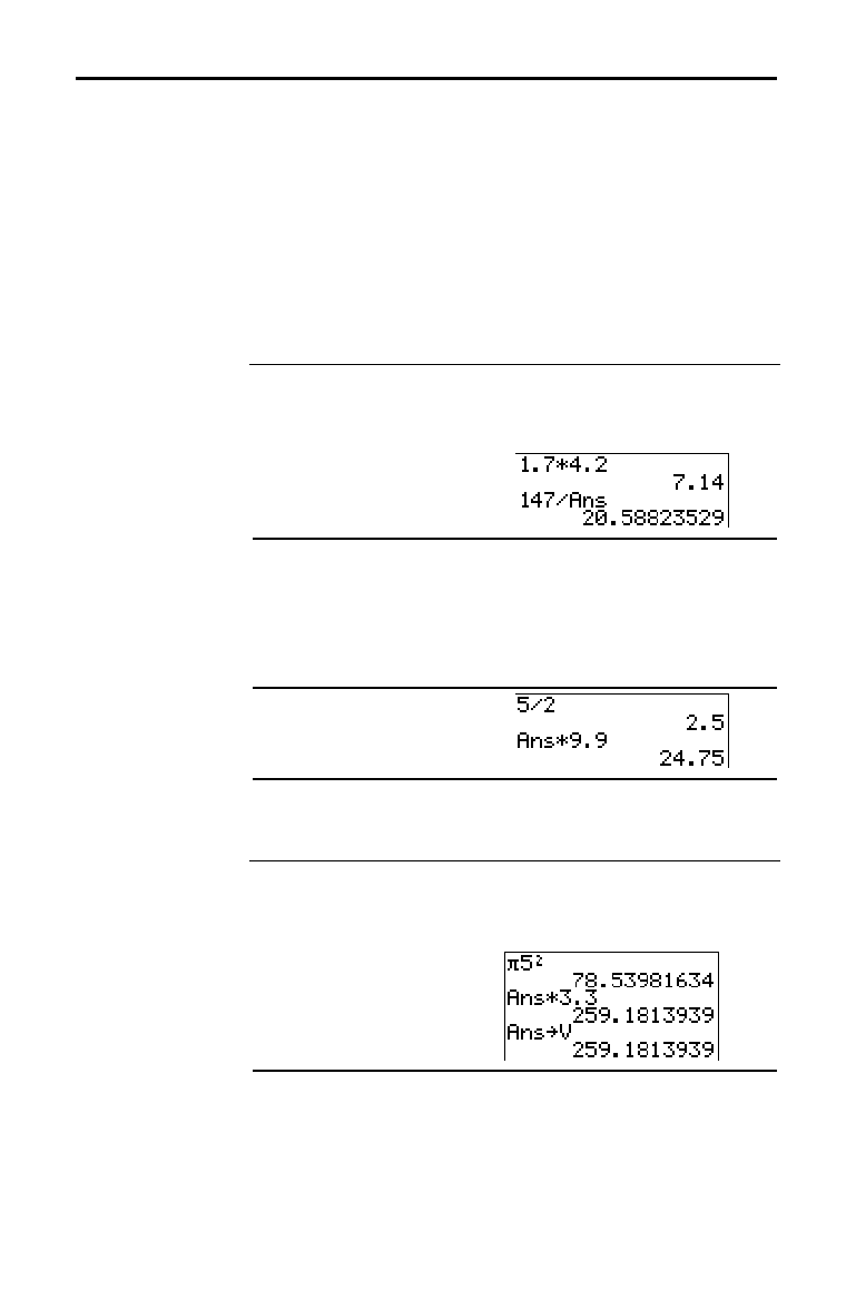
1-18 Operating the TI
-
83
8301OPER.DOC TI-83 international English Bob Fedorisko Revised: 02/19/01 12:09 PM Printed: 02/19/01 1:34
PM Page 18 of 24
When an expression is evaluated successfully from the
home screen or from a program, the TI
.
83 stores the
answer to a storage area called
Ans (last answer). Ans may
be a real or complex number, a list, a matrix, or a string.
When you turn off the TI
.
83, the value in
Ans is retained in
memory.
You can use the variable
Ans to represent the last answer in
most places. Press
y
[
ANS
] to copy the variable name Ans
to the cursor location. When the expression is evaluated, the
TI
.
83 uses the value of
Ans in the calculation.
Calculate the area of a garden plot 1.7 meters by 4.2 meters.
Then calculate the yield per square meter if the plot produces a
total of 147 tomatoes.
1
Ë
7
¯
4
Ë
2
Í
147
¥
y
[
ANS
]
Í
You can use Ans as the first entry in the next expression
without entering the value again or pressing
y
[
ANS
]. On
a blank line on the home screen, enter the function. The
TI
.
83 pastes the variable name
Ans to the screen, then the
function.
5
¥
2
Í
¯
9
Ë
9
Í
To store an answer, store Ans to a variable before you
evaluate another expression.
Calculate the area of a circle of radius 5 meters. Next, calculate
the volume of a cylinder of radius 5 meters and height 3.3 meters,
and then store the result in the variable V.
y
[
p
] 5
¡
Í
¯
3
Ë
3
Í
¿
ƒ
V
Í
Ans (Last Answer) Storage Area
Using Ans in an
Expression
Continuing an
Expression
Storing Answers

Operating the TI
-
83 1-19
8301OPER.DOC TI-83 international English Bob Fedorisko Revised: 02/19/01 12:09 PM Printed: 02/19/01 1:34
PM Page 19 of 24
You can access most TI
.
83 operations using menus. When
you press a key or key combination to display a menu, one
or more menu names appear on the top line of the screen.
•
The menu name on the left side of the top line is
highlighted. Up to seven items in that menu are
displayed, beginning with item
1, which also is
highlighted.
•
A number or letter identifies each menu item’s place in
the menu. The order is
1 through 9, then 0, then A, B, C,
and so on. The
LIST NAMES
,
PRGM EXEC
, and
PRGM
EDIT
menus only label items 1 through 9 and 0.
•
When the menu continues beyond the displayed items, a
down arrow (
$
) replaces the colon next to the last
displayed item.
•
When a menu item ends in an ellipsis, the item displays
a secondary menu or editor when you select it.
To display any other menu listed on the top line, press
~
or
|
until that menu name is highlighted. The cursor
location within the initial menu is irrelevant. The menu is
displayed with the cursor on the first item.
Note:
The Menu Map in Appendix A shows each menu, each
operation under each menu, and the key or key combination you press
to display each menu.
To scroll down the menu items, press
†
. To scroll up the
menu items, press
}
.
To page down six menu items at a time, press
ƒ
†
. To
page up six menu items at a time, press
ƒ
}
. The
green arrows on the calculator, between
†
and
}
, are the
page-down and page-up symbols.
To wrap to the last menu item directly from the first menu
item, press
}
. To wrap to the first menu item directly from
the last menu item, press
†
.
TI-83 Menus
Using a TI-83
Menu
Scrolling a Menu
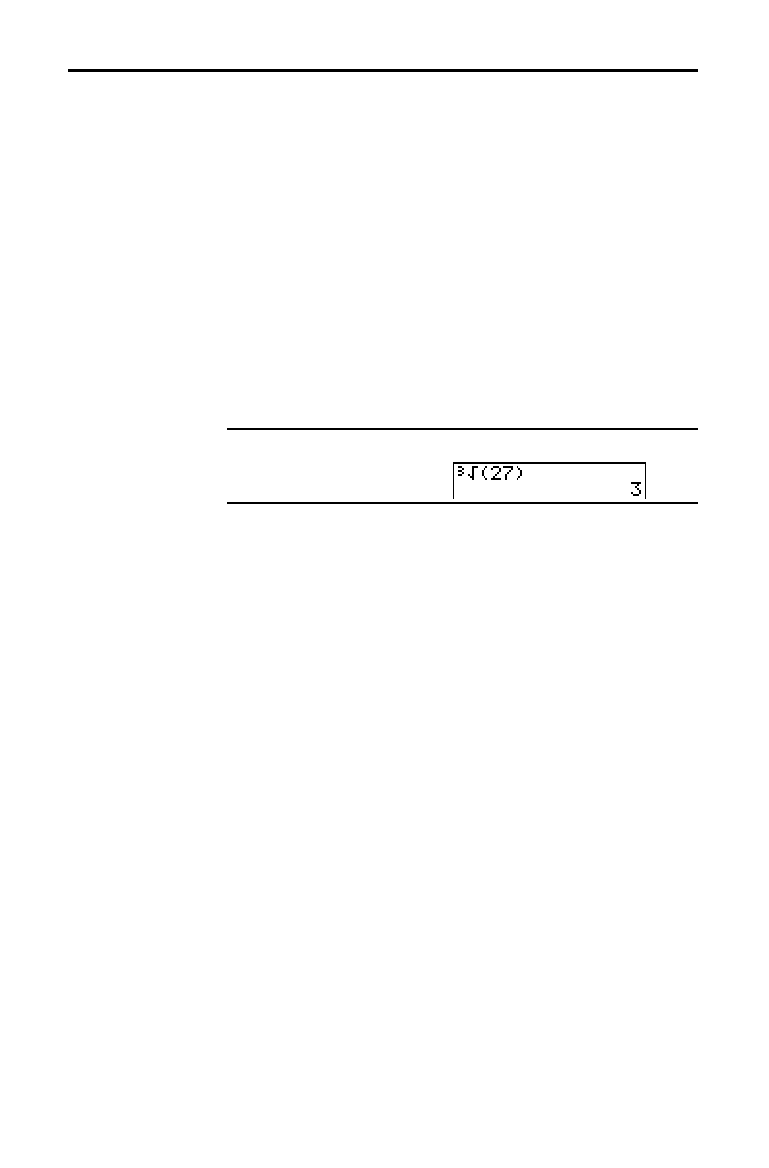
1-20 Operating the TI
-
83
8301OPER.DOC TI-83 international English Bob Fedorisko Revised: 02/19/01 12:09 PM Printed: 02/19/01 1:34
PM Page 20 of 24
You can select an item from a menu in either of two ways.
•
Press the number or letter of the item you want to
select. The cursor can be anywhere on the menu, and
the item you select need not be displayed on the screen.
•
Press
†
or
}
to move the cursor to the item you want,
and then press
Í
.
After you select an item from a menu, the TI
.
83 typically
displays the previous screen.
Note:
On the
LIST NAMES
,
PRGM EXEC
, and
PRGM EDIT
menus, only items
1
through
9
and
0
are labeled in such a way that
you can select them by pressing the appropriate number key. To move
the cursor to the first item beginning with any alpha character or
q
,
press the key combination for that alpha character or
q
. If no items
begin with that character, then the cursor moves beyond it to the next
item.
Calculate
3
‡
27.
†
†
†
Í
27
¤
Í
You can leave a menu without making a selection in any of
four ways.
•
Press
y
[
QUIT
] to return to the home screen.
•
Press
‘
to return to the previous screen.
•
Press a key or key combination for a different menu,
such as
or
y
[
LIST
].
•
Press a key or key combination for a different screen,
such as
o
or
y
[
TABLE
].
Selecting an Item
from a Menu
Leaving a Menu
without Making a
Selection
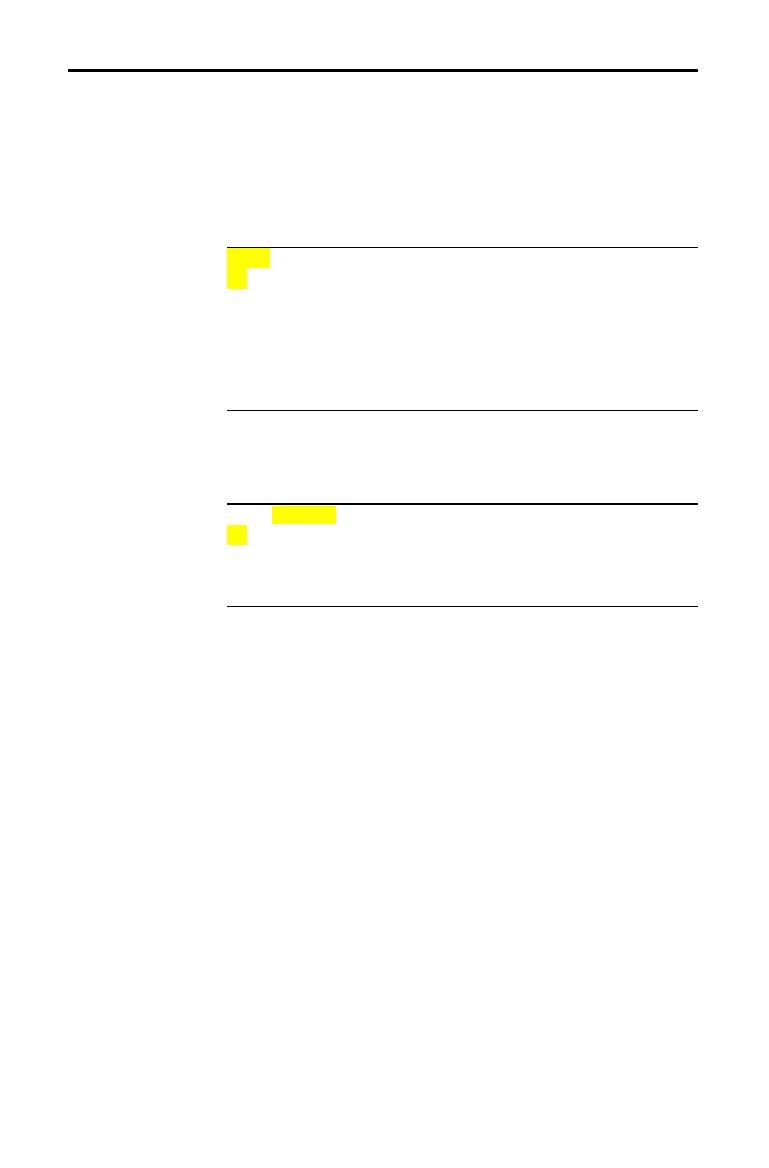
Operating the TI
-
83 1-21
8301OPER.DOC TI-83 international English Bob Fedorisko Revised: 02/19/01 12:09 PM Printed: 02/19/01 1:34
PM Page 21 of 24
You can enter the names of functions and system variables
in an expression or store to them directly.
To display the
VARS
menu, press
. All
VARS
menu
items display secondary menus, which show the names of
the system variables.
1:Window, 2:Zoom, and 5:Statistics
each access more than one secondary menu.
VARS Y-VARS
1: Window
...
X/Y
,
T/
q
, and
U/V/W
variables
2: Zoom
...
ZX/ZY
,
ZT/Z
q
, and
ZU
variables
3: GDB
...
Graph database
variables
4: Picture
...
Picture
variables
5: Statistics
...
XY
,
G
,
EQ
,
TEST
, and
PTS
variables
6: Table
...
TABLE
variables
7: String
...
String
variables
To display the
VARS Y
.
VARS
menu, press
~
.
1:Function, 2:Parametric, and 3:Polar display secondary
menus of the
Y=
function variables.
VARS Y-VARS
1: Function
...
Y
n
functions
2: Parametric
...
X
n
T
, Y
n
T
functions
3: Polar
...
r
n
functions
4: On/Off
...
Lets you select/deselect functions
Note:
The sequence variables (
u
,
v
,
w
) are located on the keyboard
as the second functions of
¬
,
−
, and
®
.
To select a variable from the
VARS
or
VARS Y
.
VARS
menu,
follow these steps.
1. Display the
VARS
or
VARS Y
.
VARS
menu.
•
Press
to display the
VARS
menu.
•
Press
~
to display the
VARS Y
.
VARS
menu.
2. Select the type of variable, such as
2:Zoom from the
VARS
menu or 3:Polar from the
VARS Y
.
VARS
menu. A
secondary menu is displayed.
3. If you selected
1:Window, 2:Zoom, or 5:Statistics from
the
VARS
menu, you can press
~
or
|
to display other
secondary menus.
4. Select a variable name from the menu. It is pasted to the
cursor location.
VARS and VARS Y-VARS Menus
VARS Menu
Selecting a
Variable from the
VARS Menu or
VARS Y-VARS
Menu

1-22 Operating the TI
-
83
8301OPER.DOC TI-83 international English Bob Fedorisko Revised: 02/19/01 12:09 PM Printed: 02/19/01 1:34
PM Page 22 of 24
The Equation Operating System (EOS
é
) defines the order
in which functions in expressions are entered and
evaluated on the TI
.
83. EOS lets you enter numbers and
functions in a simple, straightforward sequence.
EOS evaluates the functions in an expression in this order:
1 Single-argument functions that precede the
argument, such as
‡
(
, sin(, or log(
2 Functions that are entered after the argument,
such as
2
,
M
1
, !,
¡
,
r
, and conversions
3 Powers and roots, such as 2^5 or 5
x
‡
32
4 Permutations (nPr) and combinations (nCr)
5 Multiplication, implied multiplication, and
division
6 Addition and subtraction
7 Relational functions, such as > or
8 Logic operator and
9 Logic operators or and xor
Within a priority level, EOS evaluates functions from left to
right.
Calculations within parentheses are evaluated first.
Multiargument functions, such as
nDeriv(A
2
,A,6), are
evaluated as they are encountered.
Equation Operating System (EOS™)
Order of
Evaluation
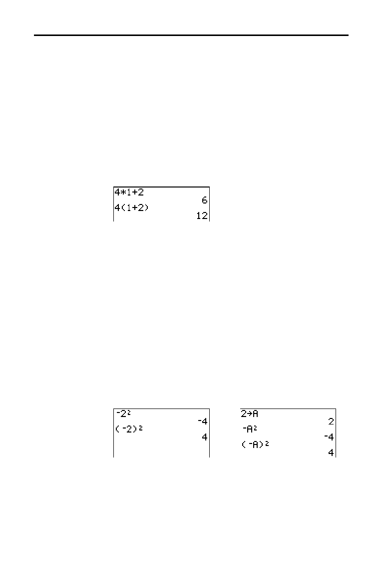
Operating the TI
-
83 1-23
8301OPER.DOC TI-83 international English Bob Fedorisko Revised: 02/19/01 12:09 PM Printed: 02/19/01 1:34
PM Page 23 of 24
The TI
.
83 recognizes implied multiplication, so you need
not press
¯
to express multiplication in all cases. For
example, the TI
.
83 interprets
2
p
, 4sin(46), 5(1+2), and (2
ä
5)7
as implied multiplication.
Note:
TI
.
83 implied multiplication rules differ from those of the TI
.
82.
For example, the TI
.
83 evaluates
1
à
2X
as
(1
à
2)
ä
X
, while the TI
.
82
evaluates
1
à
2X
as
1/(2
ä
X)
(Chapter 2).
All calculations inside a pair of parentheses are completed
first. For example, in the expression
4(1+2), EOS first
evaluates the portion inside the parentheses,
1+2, and then
multiplies the answer,
3, by 4.
You can omit the close parenthesis ( ) ) at the end of an
expression. All open parenthetical elements are closed
automatically at the end of an expression. This is also true
for open parenthetical elements that precede the store or
display-conversion instructions.
Note:
An open parenthesis following a list name, matrix name, or
Y=
function name does not indicate implied multiplication. It specifies
elements in the list (Chapter 11) or matrix (Chapter 10) and specifies a
value for which to solve the
Y=
function.
To enter a negative number, use the negation key. Press
Ì
and then enter the number. On the TI
.
83, negation is in the
third level in the EOS hierarchy. Functions in the first
level, such as squaring, are evaluated before negation.
For example,
M
X
2
, evaluates to a negative number (or 0).
Use parentheses to square a negative number.
Note:
Use the
¹
key for subtraction and the
Ì
key for negation. If
you press
¹
to enter a negative number, as in
9
¯
¹
7
, or if you
press
Ì
to indicate subtraction, as in
9
Ì
7
, an error occurs. If you
press
ƒ
A
Ì
ƒ
B
, it is interpreted as implied multiplication
(
A
ä
M
B
).
Implied
Multiplication
Parentheses
Negation

1-24 Operating the TI
-
83
8301OPER.DOC TI-83 international English Bob Fedorisko Revised: 02/19/01 12:09 PM Printed: 02/19/01 1:34
PM Page 24 of 24
The TI
.
83 detects errors while performing these tasks.
•
Evaluating an expression
•
Executing an instruction
•
Plotting a graph
•
Storing a value
When the TI
.
83 detects an error, it returns an error
message as a menu title, such as
ERR:SYNTAX
or
ERR:DOMAIN
. Appendix B describes each error type and
possible reasons for the error.
•
If you select
1:Quit (or press
y
[
QUIT
] or
‘
), then
the home screen is displayed.
•
If you select
2:Goto, then the previous screen is
displayed with the cursor at or near the error location.
Note
: If a syntax error occurs in the contents of a Y= function during
program execution, then the
Goto
option returns to the Y= editor, not
to the program.
To correct an error, follow these steps.
1. Note the error type (
ERR:
error type
).
2. Select
2:Goto, if it is available. The previous screen is
displayed with the cursor at or near the error location.
3. Determine the error. If you cannot recognize the error,
refer to Appendix B.
4. Correct the expression.
Error Conditions
Diagnosing an
Error
Correcting an
Error
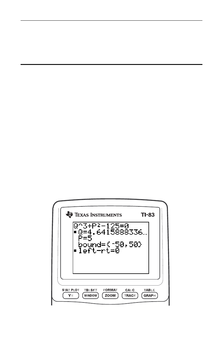
Math, Angle, and Test Operations 2-1
2
Math, An
g
le, and Test
Operations
Getting Started: Coin Flip
................................
2-2
Keyboard Math Operations
..............................
2-3
MATH
Operations
........................................
2-5
Using the Equation Solver
...............................
2-8
MATH NUM
(Number) Operations
........................
2-13
Entering and Using Complex Numbers
...................
2-16
MATH CPX
(Complex) Operations
.......................
2-18
MATH PRB
(Probability) Operations
.....................
2-20
ANGLE
Operations
.......................................
2-23
TEST
(Relational) Operations
............................
2-24
TEST LOGIC
(Boolean) Operations
......................
2-26
Contents
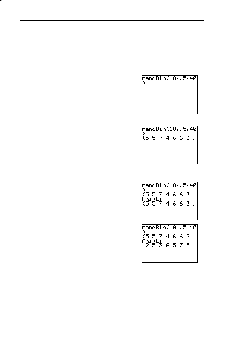
2-2 Math, Angle, and Test Operations
8302MATH.DOC TI-83 international English Bob Fedorisko Revised: 02/19/01 12:12 PM Printed: 02/19/01 2:27
PM Page 2 of 26
Getting Started is a fast-paced introduction. Read the chapter for details.
Suppose you want to model flipping a fair coin 10 times. You want to track
how many of those 10 coin flips result in heads. You want to perform this
simulation 40 times. With a fair coin, the probability of a coin flip resulting in
heads is 0.5 and the probability of a coin flip resulting in tails is 0.5.
1. Begin on the home screen. Press
|
to
display the
MATH PRB
menu. Press 7 to
select
7:randBin( (random Binomial).
randBin( is pasted to the home screen. Press
10 to enter the number of coin flips. Press
¢
. Press
Ë
5 to enter the probability of
heads. Press
¢
. Press
40 to enter the
number of simulations. Press
¤
.
2. Press
Í
to evaluate the expression. A
list of 40 elements is displayed. The list
contains the count of heads resulting from
each set of 10 coin flips. The list has 40
elements because this simulation was
performed 40 times. In this example, the
coin came up heads five times in the first
set of 10 coin flips, five times in the second
set of 10 coin flips, and so on.
3. Press
¿
y
ã
L1ä
Í
to store the data
to the list name
L
1
. You then can use the
data for another activity, such as plotting a
histogram (Chapter 12).
4. Press
~
or
|
to view the additional counts
in the list. Ellipses (
...) indicate that the list
continues beyond the screen.
Note:
Since
randBin(
generates random
numbers, your list elements may differ from those
in the example.
Getting Started: Coin Flip
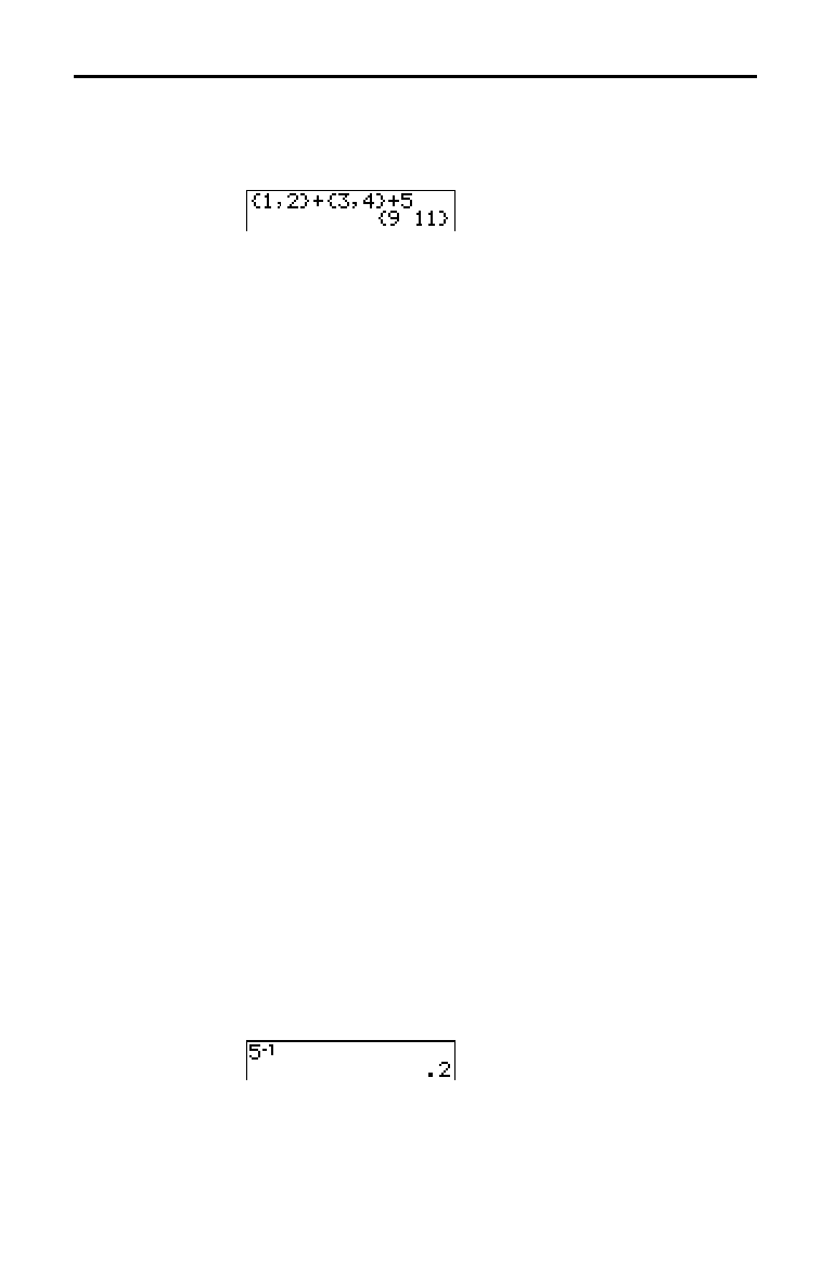
Math, Angle, and Test Operations 2-3
Math operations that are valid for lists return a list
calculated element by element. If you use two lists in the
same expression, they must be the same length.
You can use + (addition,
Ã
),
N
(subtraction,
¹
),
ä
(multiplication,
¯
), and
à
(division,
¥
) with real and
complex numbers, expressions, lists, and matrices. You
cannot use
à
with matrices.
valueA
+
valueB valueA
N
valueB
valueA
ä
valueB valueA
à
valueB
You can use the trigonometric (trig) functions (sine,
˜
;
cosine,
™
; and tangent,
š
) with real numbers,
expressions, and lists. The current angle mode setting
affects interpretation. For example,
sin(30) in Radian mode
returns
L
.9880316241
; in Degree mode it returns .5.
sin(
value
) cos(
value
) tan(
value
)
You can use the inverse trig functions (arcsine,
y
[
SIN
L
1
];
arccosine,
y
[
COS
L
1
]; and arctangent,
y
[
TAN
L
1
]) with
real numbers, expressions, and lists. The current angle
mode setting affects interpretation.
sin
L
1
(
value
) cos
L
1
(
value
) tan
L
1
(
value
)
Note:
The trig functions do not operate on complex numbers.
You can use ^ (power,
›
),
2
(square,
¡
), and
‡
(
(square
root,
y
[
‡
]) with real and complex numbers, expressions,
lists, and matrices. You cannot use
‡
(
with matrices.
value
^
power value
2
‡
(
value
)
You can use
L
1
(inverse,
—
) with real and complex
numbers, expressions, lists, and matrices. The
multiplicative inverse is equivalent to the reciprocal, 1
à
x
.
value
L
1
Keyboard Math Operations
Using Lists with
Math Operations
+ (Addition),
N
(Subtraction),
ä
(Multiplication),
à
(Division)
Trigonometric
Functions
^ (Power),
2
(Square),
‡
( (Square Root)
L
1
(Inverse)
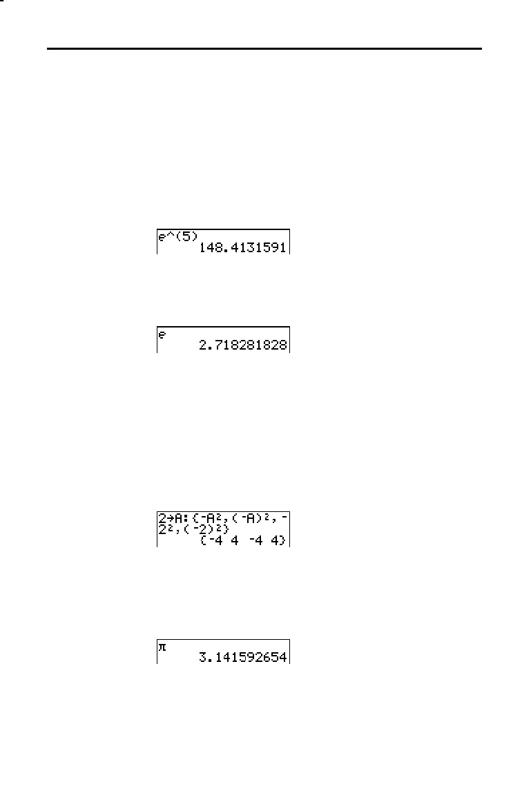
2-4 Math, Angle, and Test Operations
8302MATH.DOC TI-83 international English Bob Fedorisko Revised: 02/19/01 12:12 PM Printed: 02/19/01 2:27
PM Page 4 of 26
You can use log( (logarithm,
«
), 10^( (power of 10,
y
[
10
x
]), and ln( (natural log,
µ
) with real or complex
numbers, expressions, and lists.
log(
value
) 10^(
power
)ln(
value
)
e^(
(exponential,
y
ã
e
x
]) returns the constant e raised to
a power. You can use
e^( with real or complex numbers,
expressions, and lists.
e^(
power
)
e (constant,
y
[
e
]) is stored as a constant on the TI
-
83.
Press
y
[
e
] to copy e to the cursor location. In
calculations, the TI
-
83 uses 2.718281828459 for
e.
M
(negation,
Ì
) returns the negative of
value
. You can use
M
with real or complex numbers, expressions, lists, and
matrices.
M
value
EOS rules (Chapter 1) determine when negation is
evaluated. For example,
L
A
2
returns a negative number,
because squaring is evaluated before negation. Use
parentheses to square a negated number, as in
(
L
A)
2
.
Note:
On the TI
-
83, the negation symbol (
M
) is shorter and higher than
the subtraction sign (
N
), which is displayed when you press
¹
.
p
(Pi,
y
[
p
]) is stored as a constant in the TI
-
83. In
calculations, the TI
-
83 uses 3.1415926535898 for
p
.
log(,
10^(,
ln(
e^( (Exponential)
e (Constant)
L
(Negation)
p
(Pi)
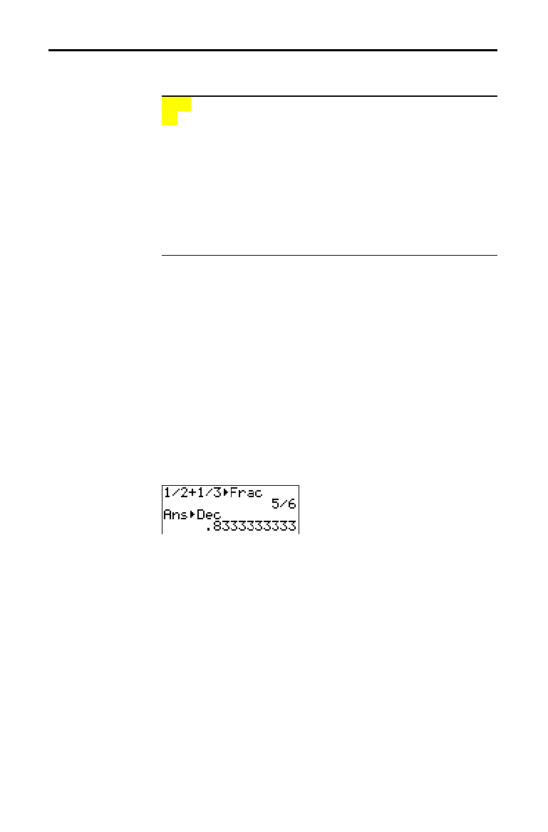
Math, Angle, and Test Operations 2-5
To display the
MATH
menu, press
.
MATH NUM CPX PRB
1:
4
Frac
Displays the answer as a fraction.
2:
4
Dec
Displays the answer as a decimal.
3:
3
Calculates the cube.
4:
3
‡
(
Calculates the cube root.
5:
x
‡
Calculates the
x
th
root.
6: fMin(
Finds the minimum of a function.
7: fMax(
Finds the maximum of a function.
8: nDeriv(
Computes the numerical derivative.
9: fnInt(
Computes the function integral.
0: Solver
...
Displays the equation solver.
4
Frac
(display as a fraction) displays an answer as its
rational equivalent. You can use
4
Frac
with real or complex
numbers, expressions, lists, and matrices. If the answer
cannot be simplified or the resulting denominator is more
than three digits, the decimal equivalent is returned. You
can only use
4
Frac
following
value
.
value
4
Frac
4
Dec
(display as a decimal) displays an answer in decimal
form. You can use
4
Dec
with real or complex numbers,
expressions, lists, and matrices. You can only use
4
Dec
following
value
.
value
4
Dec
MATH Operations
MATH Menu
4
Frac,
4
Dec
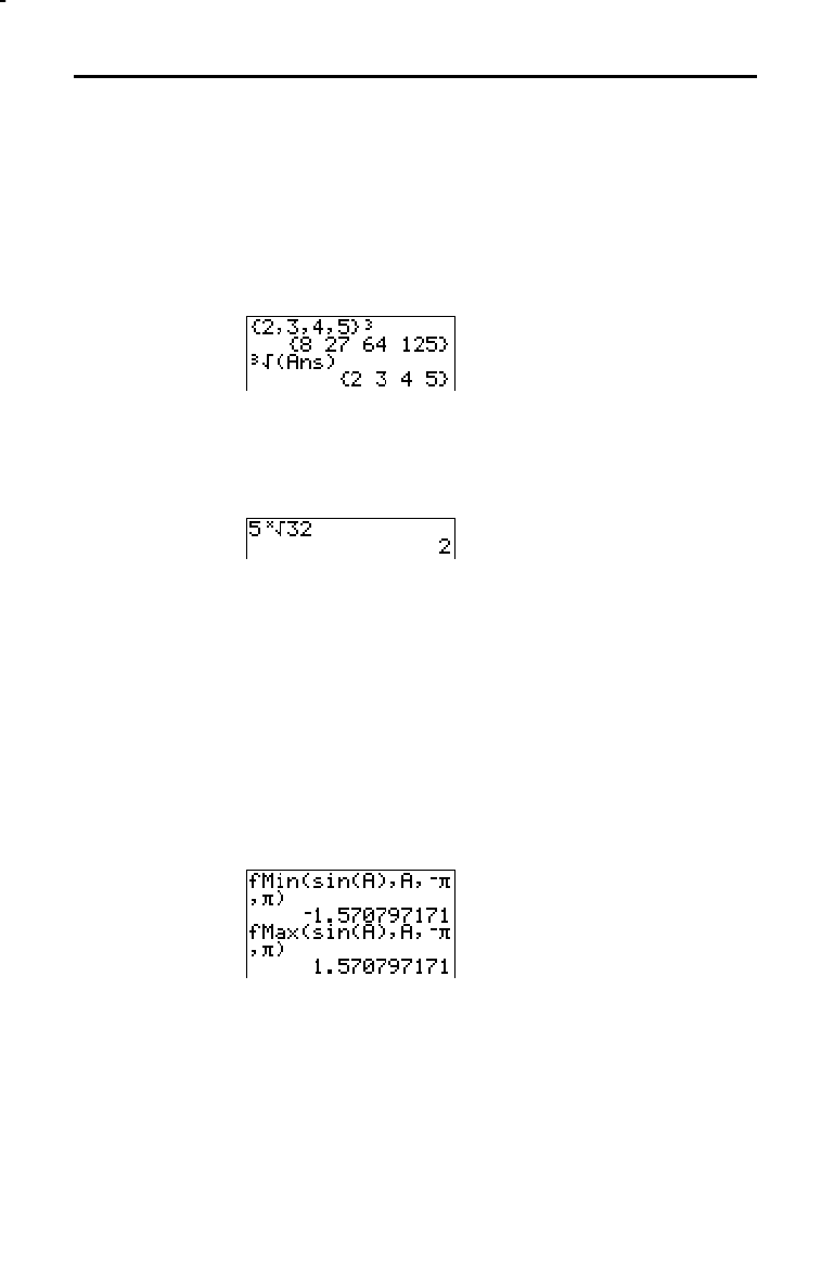
2-6 Math, Angle, and Test Operations
8302MATH.DOC TI-83 international English Bob Fedorisko Revised: 02/19/01 12:12 PM Printed: 02/19/01 2:27
PM Page 6 of 26
3
(cube) returns the cube of
value
. You can use
3
with real
or complex numbers, expressions, lists, and square
matrices.
value
3
3
‡
(
(cube root) returns the cube root of
value
. You can use
3
‡
(
with real or complex numbers, expressions, and lists.
3
‡
(
value
)
x
‡
(
x
th
root) returns the
x
th
root
of
value
. You can use
x
‡
with real or complex numbers, expressions, and lists.
x
th
root
x
‡
value
fMin( (function minimum) and fMax( (function maximum)
return the value at which the local minimum or local
maximum value of
expression
with respect to
variable
occurs, between
lower
and
upper
values for
variable
.
fMin(
and fMax( are not valid in
expression
. The accuracy is
controlled by
tolerance
(if not specified, the default is
1
â
L
5).
fMin(
expression
,
variable
,
lower
,
upper
[
,
tolerance
]
)
fMax(
expression
,
variable
,
lower
,
upper
[
,
tolerance
]
)
Note:
In this guidebook, optional arguments and the commas that
accompany them are enclosed in brackets ([ ]).
3
(Cube),
3
‡
( (Cube Root)
x
‡
(Root)
fMin(,
fMax(
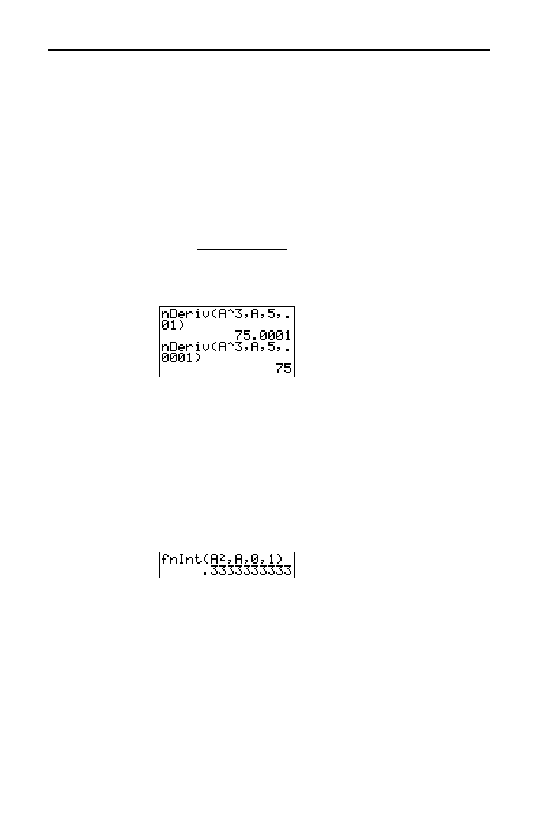
Math, Angle, and Test Operations 2-7
nDeriv( (numerical derivative) returns an approximate
derivative of
expression
with respect to
variable
, given the
value
at which to calculate the derivative and
H
(if not
specified, the default is 1
â
L
3). nDeriv( is valid only for real
numbers.
nDeriv(
expression
,
variable
,
value
[
,
H
]
)
nDeriv( uses the symmetric difference quotient method,
which approximates the numerical derivative value as the
slope of the secant line through these points.
f
(
x
+
H
)
N
f(
x
NH
)
f
¢
(
x
) =
2
H
As
H
becomes smaller, the approximation usually becomes
more accurate.
You can use nDeriv( once in
expression
. Because of the
method used to calculate
nDeriv(, the TI
-
83 can return a
false derivative value at a nondifferentiable point.
fnInt( (function integral) returns the numerical integral
(Gauss-Kronrod method) of
expression
with respect to
variable
, given
lower
limit,
upper
limit, and a
tolerance
(if
not specified, the default is 1
â
L
5). fnInt( is valid only for real
numbers.
fnInt(
expression
,
variable
,
lower
,
upper
[
,
tolerance
]
)
Tip:
To speed the drawing of integration graphs (when
fnInt(
is used
in a Y= equation), increase the value of the
Xres
window variable
before you press
s
.
nDeriv(
fnInt(
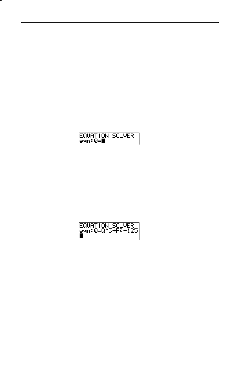
2-8 Math, Angle, and Test Operations
8302MATH.DOC TI-83 international English Bob Fedorisko Revised: 02/19/01 12:12 PM Printed: 02/19/01 2:27
PM Page 8 of 26
Solver displays the equation solver, in which you can solve
for any variable in an equation. The equation is assumed to
be equal to zero.
Solver is valid only for real numbers.
When you select
Solver, one of two screens is displayed.
•
The equation editor (see step 1 picture below) is
displayed when the equation variable
eqn is empty.
•
The interactive solver editor (see step 3 picture on page
2
.
9) is displayed when an equation is stored in
eqn.
To enter an expression in the equation solver, assuming
that the variable
eqn is empty, follow these steps.
1. Select
0:Solver from the
MATH
menu to display the
equation editor.
2. Enter the expression in any of three ways.
•
Enter the expression directly into the equation
solver.
•
Paste a
Y=
variable name from the
VARS Y
.
VARS
menu to the equation solver.
•
Press
y
[
RCL
], paste a
Y=
variable name from the
VARS Y
.
VARS
menu, and press
Í
. The
expression is pasted to the equation solver.
The expression is stored to the variable
eqn as you
enter it.
Using the Equation Solver
Solver
Entering an
Expression in the
Equation Solver
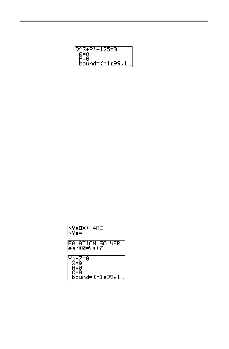
Math, Angle, and Test Operations 2-9
3. Press
Í
or
†
. The interactive solver editor is
displayed.
•
The equation stored in
eqn is set equal to zero and
displayed on the top line.
•
Variables in the equation are listed in the order in
which they appear in the equation. Any values stored
to the listed variables also are displayed.
•
The default lower and upper bounds appear in the
last line of the editor (
bound={
L
1
å
99,1
å
99}).
•
A
$
is displayed in the first column of the bottom line
if the editor continues beyond the screen.
Tip:
To use the solver to solve an equation such as
K=.5MV
2
, enter
eqn:0=K
N
.5MV
2
in the equation editor.
When you enter or edit a value for a variable in the
interactive solver editor, the new value is stored in
memory to that variable.
You can enter an expression for a variable value. It is
evaluated when you move to the next variable.
Expressions must resolve to real numbers at each step
during the iteration.
You can store equations to any
VARS Y
.
VARS
variables,
such as
Y
1
or r
6
, and then reference the variables in the
equation. The interactive solver editor displays all
variables of all
Y=
functions referenced in the equation.
Entering and
Editing Variable
Values
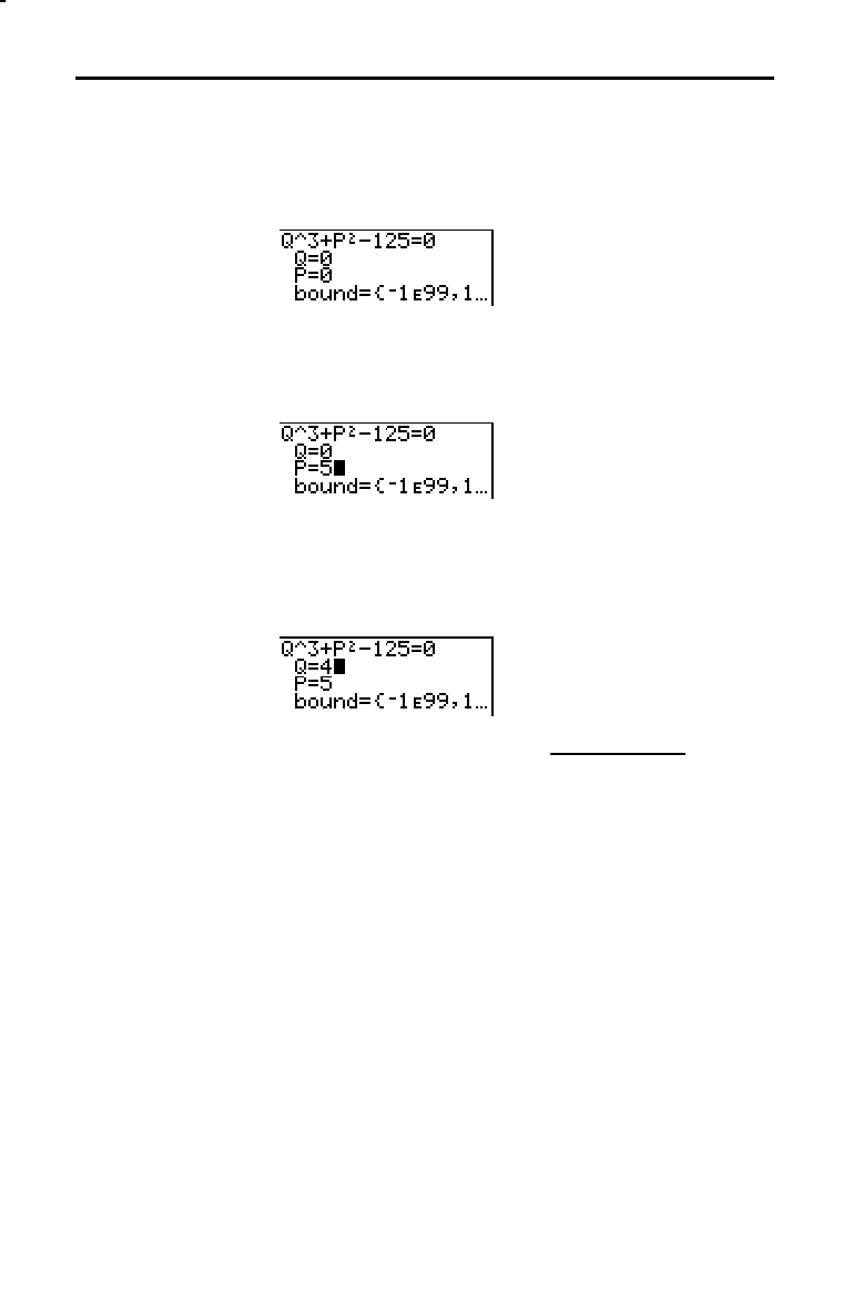
2-10 Math, Angle, and Test Operations
8302MATH.DOC TI-83 international English Bob Fedorisko Revised: 02/19/01 12:12 PM Printed: 02/19/01 2:27
PM Page 10 of 26
To solve for a variable using the equation solver after an
equation has been stored to
eqn, follow these steps.
1. Select
0:Solver from the
MATH
menu to display the
interactive solver editor, if not already displayed.
2. Enter or edit the value of each known variable. All
variables, except the unknown variable, must contain a
value. To move the cursor to the next variable, press
Í
or
†
.
3. Enter an initial guess for the variable for which you are
solving. This is optional, but it may help find the
solution more quickly. Also, for equations with multiple
roots, the TI
-
83 will attempt to display the solution that
is closest to your guess.
The default guess is calculated as
(
upper +lower
)
2
.
Solving for a
Variable in the
Equation Solver
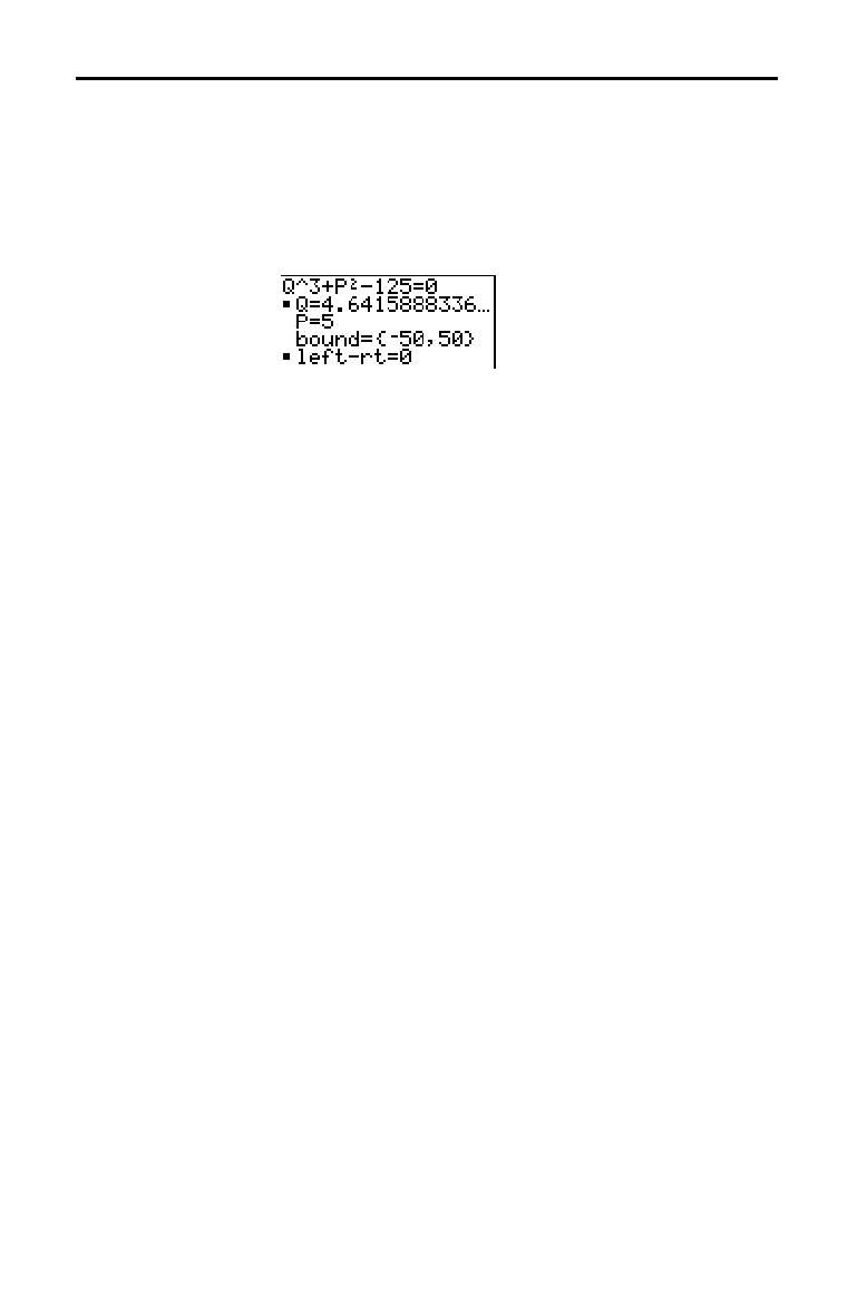
Math, Angle, and Test Operations 2-11
4. Edit
bound={
lower
,
upper
}.
lower
and
upper
are the
bounds between which the TI
-
83 searches for a solution.
This is optional, but it may help find the solution more
quickly. The default is
bound={
L
1
å
99,1
å
99}.
5. Move the cursor to the variable for which you want to
solve and press
ƒ
[
SOLVE
] (above the
Í
key).
•
The solution is displayed next to the variable for
which you solved. A solid square in the first column
marks the variable for which you solved and
indicates that the equation is balanced. An ellipsis
shows that the value continues beyond the screen.
Note:
When a number continues beyond the screen, be sure to
press
~
to scroll to the end of the number to see whether it
ends with a negative or positive exponent. A very small number
may appear to be a large number until you scroll right to see
the exponent.
•
The values of the variables are updated in memory.
•
left
N
rt=
diff
is displayed in the last line of the editor.
diff
is the difference between the left and right sides
of the equation. A solid square in the first column
next to
left
N
rt= indicates that the equation has been
evaluated at the new value of the variable for which
you solved.
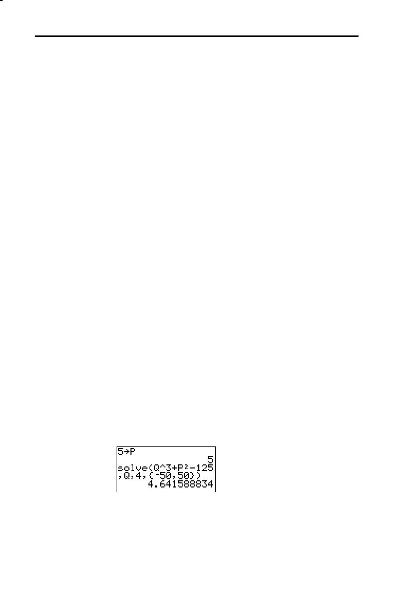
2-12 Math, Angle, and Test Operations
8302MATH.DOC TI-83 international English Bob Fedorisko Revised: 02/19/01 12:12 PM Printed: 02/19/01 2:27
PM Page 12 of 26
To edit or replace an equation stored to eqn when the
interactive equation solver is displayed, press
}
until the
equation editor is displayed. Then edit the equation.
Some equations have more than one solution. You can
enter a new initial guess (page 2
.
10) or new bounds
(page 2
.
11) to look for additional solutions.
After you solve for a variable, you can continue to explore
solutions from the interactive solver editor. Edit the values
of one or more variables. When you edit any variable value,
the solid squares next to the previous solution and
left
N
rt=
diff
disappear. Move the cursor to the variable for
which you now want to solve and press
ƒ
[
SOLVE
].
The TI
-
83 solves equations through an iterative process. To
control that process, enter bounds that are relatively close
to the solution and enter an initial guess within those
bounds. This will help to find a solution more quickly. Also,
it will define which solution you want for equations with
multiple solutions.
The function
solve( is available only from
CATALOG
or
from within a program. It returns a solution (root) of
expression
for
variable
, given an initial
guess
, and
lower
and
upper
bounds within which the solution is sought. The
default for
lower
is
L
1
â
99. The default for
upper
is 1
â
99.
solve( is valid only for real numbers.
solve(
expression
,
variable
,
guess
[
,{
lower
,
upper
}])
expression
is assumed equal to zero. The value of
variable
will not be updated in memory.
guess
may be a value or a
list of two values. Values must be stored for every variable
in
expression
, except
variable
, before
expression
is
evaluated.
lower
and
upper
must be entered in list format.
Editing an
Equation Stored
to eqn
Equations with
Multiple Roots
Further Solutions
Controlling the
Solution for
Solver or solve(
Using solve( on
the Home Screen
or from a
Program
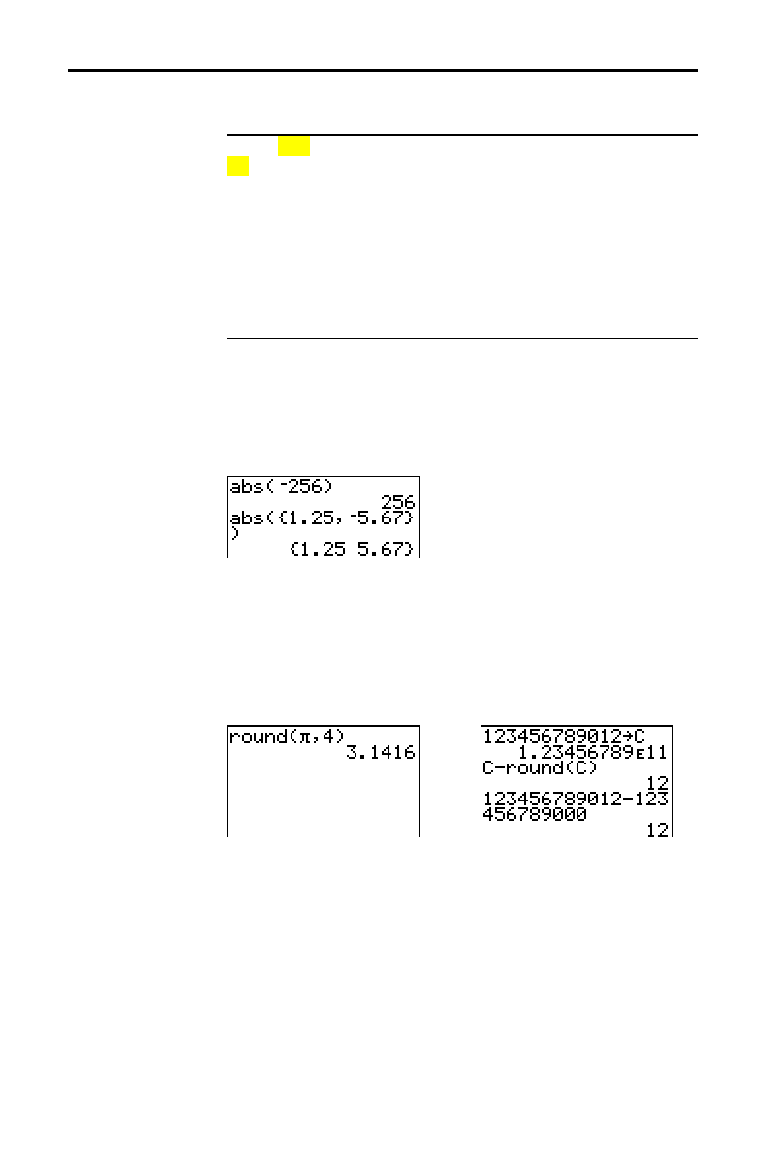
Math, Angle, and Test Operations 2-13
To display the
MATH NUM
menu, press
~
.
MATH NUM CPX PRB
1: abs(
Absolute value
2: round(
Round
3: iPart(
Integer part
4: fPart(
Fractional part
5: int(
Greatest integer
6: min(
Minimum value
7: max(
Maximum value
8: lcm(
Least common multiple
9: gcd(
Greatest common divisor
abs( (absolute value) returns the absolute value of real or
complex (modulus) numbers, expressions, lists, and
matrices.
abs(
value
)
Note:
abs(
is also available on the
MATH CPX
menu.
round( returns a number, expression, list, or matrix
rounded to
#decimals
(
9). If
#decimals
is omitted,
value
is rounded to the digits that are displayed, up to 10 digits.
round(
value
[
,
#decimals
]
)
MATH NUM (Number) Operations
MATH NUM Menu
abs(
round(
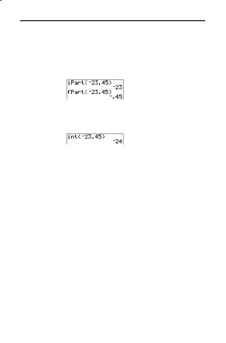
2-14 Math, Angle, and Test Operations
8302MATH.DOC TI-83 international English Bob Fedorisko Revised: 02/19/01 12:12 PM Printed: 02/19/01 2:27
PM Page 14 of 26
iPart( (integer part) returns the integer part or parts of real
or complex numbers, expressions, lists, and matrices.
iPart(
value
)
fPart( (fractional part) returns the fractional part or parts of
real or complex numbers, expressions, lists, and matrices.
fPart(
value
)
int( (greatest integer) returns the largest integer
real or
complex numbers, expressions, lists, and matrices.
int(
value
)
Note:
For a given
value
, the result of
int(
is the same as the result of
iPart(
for nonnegative numbers and negative integers, but one integer
less than the result of
iPart(
for negative noninteger numbers.
iPart(,
fPart(
int(
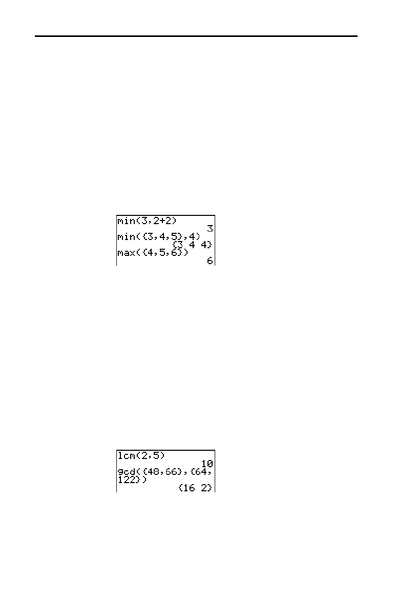
Math, Angle, and Test Operations 2-15
min( (minimum value) returns the smaller of
valueA
and
valueB
or the smallest element in
list
. If
listA
and
listB
are
compared,
min( returns a list of the smaller of each pair of
elements. If
list
and
value
are compared,
min( compares
each element in
list
with
value
.
max( (maximum value) returns the larger of
valueA
and
valueB
or the largest element in
list
. If
listA
and
listB
are
compared,
max( returns a list of the larger of each pair of
elements. If
list
and
value
are compared,
max( compares
each element in
list
with
value
.
min(
valueA
,
valueB
) max(
valueA
,
valueB
)
min(
list
) max(
list
)
min(
listA
,
listB
) max(
listA
,
listB
)
min(
list
,
value
) max(
list
,
value
)
Note:
min(
and
max(
also are available on the
LIST MATH
menu.
lcm( returns the least common multiple of
valueA
and
valueB
, both of which must be nonnegative integers. When
listA
and
listB
are specified,
lcm( returns a list of the lcm
of each pair of elements. If
list
and
value
are specified,
lcm( finds the lcm of each element in
list
and
value
.
gcd( returns the greatest common divisor of
valueA
and
valueB
, both of which must be nonnegative integers. When
listA
and
listB
are specified,
gcd( returns a list of the gcd
of each pair of elements. If
list
and
value
are specified,
gcd( finds the gcd of each element in
list
and
value
.
lcm(
valueA
,
valueB
) gcd(
valueA
,
valueB
)
lcm(
listA
,
listB
) gcd(
listA
,
listB
)
lcm(
list
,
value
) gcd(
list
,
value
)
min(,
max(
lcm(,
gcd(
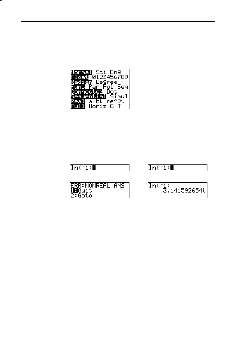
2-16 Math, Angle, and Test Operations
8302MATH.DOC TI-83 international English Bob Fedorisko Revised: 02/19/01 12:12 PM Printed: 02/19/01 2:27
PM Page 16 of 26
The TI
-
83 displays complex numbers in rectangular form
and polar form. To select a complex-number mode, press
z
, and then select either of the two modes.
•
a+b
i
(rectangular-complex mode)
•
re^
q
i
(polar-complex mode)
On the TI
-
83, complex numbers can be stored to variables.
Also, complex numbers are valid list elements.
In
Real mode, complex-number results return an error,
unless you entered a complex number as input. For
example, in
Real mode ln(
L
1) returns an error; in a+b
i
mode
ln(
L
1) returns an answer.
Real mode a+b
i
mode
$$
Complex numbers are stored in rectangular form, but you
can enter a complex number in rectangular form or polar
form, regardless of the mode setting. The components of
complex numbers can be real numbers or expressions that
evaluate to real numbers; expressions are evaluated when
the command is executed.
Radian mode is recommended for complex number
calculations. Internally, the TI
-
83 converts all entered trig
values to radians, but it does not convert values for
exponential, logarithmic, or hyperbolic functions.
In degree mode, complex identities such as
e
^(
i
q
) = cos(
q
) +
i
sin(
q
) are not generally true because
the values for cos and sin are converted to radians, while
those for e^() are not. For example,
e
^(
i
45) = cos(45) +
i
sin(45) is treated internally as
e
^(
i
45) = cos(
p
/4) +
i
sin(
p
/4). Complex identities are
always true in radian mode.
Entering and Using Complex Numbers
Complex-Number
Modes
Entering
Complex
Numbers
Note about
Radian versus
Degree Mode
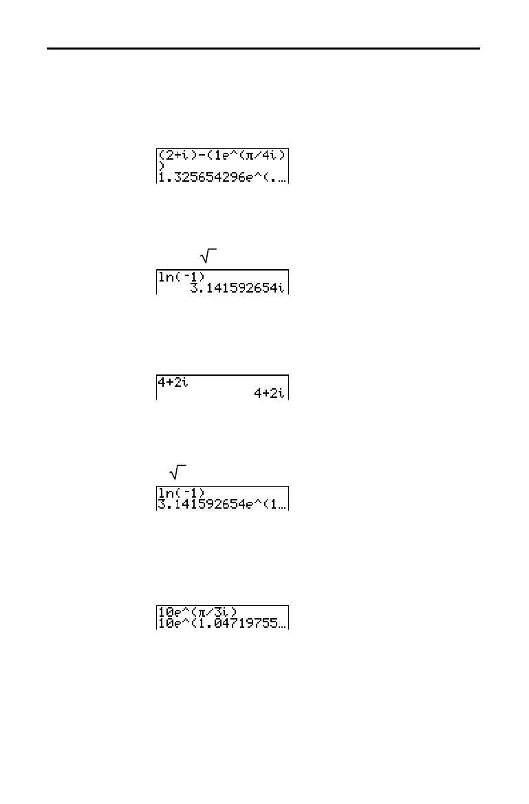
Math, Angle, and Test Operations 2-17
Complex numbers in results, including list elements, are
displayed in either rectangular or polar form, as specified
by the mode setting or by a display conversion instruction
(page 2
.
19). In the example below,
re^
q
i
and
Radian modes
are set.
Rectangular-complex mode recognizes and displays a
complex number in the form
a+b
i
, where
a
is the real
component,
b
is the imaginary component, and
i
is a constant
equal to
-1
.
To enter a complex number in rectangular form, enter the
value of
a
(
real component
), press
Ã
or
¹
, enter the value
of
b
(
imaginary component
), and press
y
[
i
] (constant).
real component
(
+ or
N
)
imaginary componenti
Polar-complex mode recognizes and displays a complex
number in the form
re^
q
i
, where
r
is the magnitude,
e
is the
base of the natural log,
q
is the angle, and
i
is a constant equal
to
-1
.
To enter a complex number in polar form, enter the value
of
r
(
magnitude
), press
y
[
e
x
] (exponential function),
enter the value of
q
(
angle
), press
y
[
i
] (constant), and
then press
¤
.
magnitude
e^(
angle
i
)
Interpreting
Complex Results
Rectangular-
Complex Mode
Polar-Complex
Mode
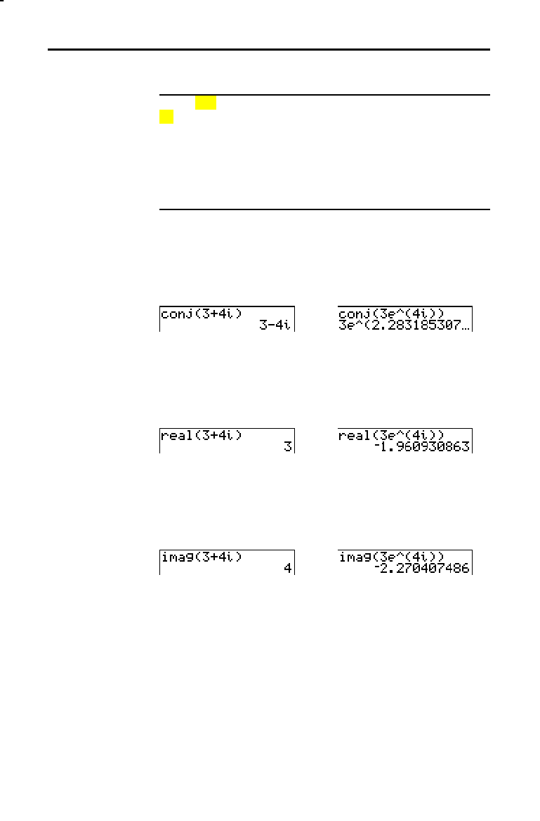
2-18 Math, Angle, and Test Operations
8302MATH.DOC TI-83 international English Bob Fedorisko Revised: 02/19/01 12:12 PM Printed: 02/19/01 2:27
PM Page 18 of 26
To display the
MATH CPX
menu, press
~
~
.
MATH NUM CPX PRB
1: conj(
Returns the complex conjugate.
2: real(
Returns the real part.
3: imag(
Returns the imaginary part.
4: angle(
Returns the polar angle.
5: abs(
Returns the magnitude (modulus).
6:
4
Rect
Displays the result in rectangular form.
7:
4
Polar
Displays the result in polar form.
conj( (conjugate) returns the complex conjugate of a
complex number or list of complex numbers.
conj(
a
+
b
i
) returns
aNb
i
in a+b
i
mode.
conj(
r
e^(
q
i
)) returns
r
e^(
Lq
i
) in re^
q
i
mode.
real( (real part) returns the real part of a complex number
or list of complex numbers.
real(
a
+
b
i
) returns
a
.
real(
r
e^(
q
i
)) returns
r
ä
cos
(
q
).
imag( (imaginary part) returns the imaginary (nonreal) part
of a complex number or list of complex numbers.
imag(
a
+
b
i
) returns
b
.
imag(
r
e^(
q
i
)) returns
r
ä
sin(
q
)
.
MATH CPX (Complex) Operations
MATH CPX Menu
conj(
real(
imag(
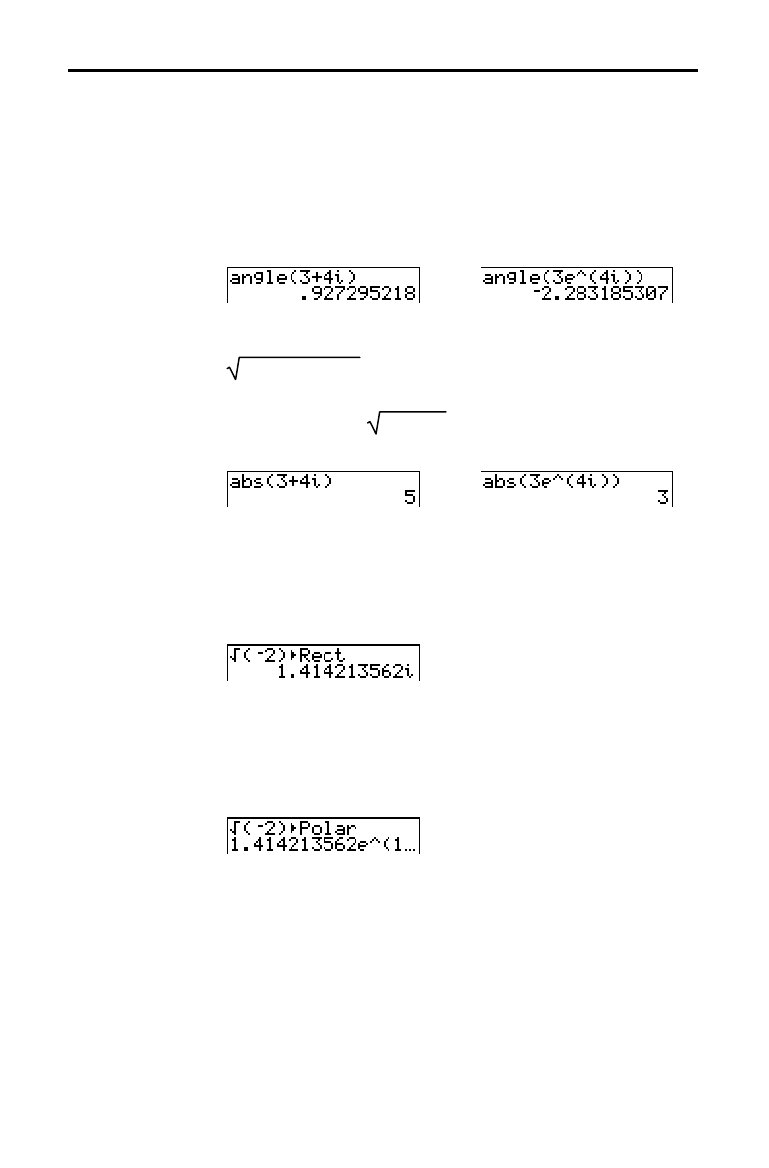
Math, Angle, and Test Operations 2-19
angle( returns the polar angle of a complex number or list
of complex numbers, calculated as tan
L
1
(b/a), where b is
the imaginary part and a is the real part. The calculation is
adjusted by +
p
in the second quadrant or
Np
in the third
quadrant.
angle(
a
+
bi
) returns
tan
L
1
(b/a)
.
angle(
r
e^(
q
i
)) returns
q
, where
Lp
<
q
<
p
.
abs( (absolute value) returns the magnitude (modulus),
(real2+imag2)
, of a complex number or list of complex
numbers.
abs(
a
+
bi
) returns
(a2+b2)
.
abs(
r
e^(
q
i
)) returns
r
(magnitude).
4
Rect
(display as rectangular) displays a complex result in
rectangular form. It is valid only at the end of an
expression. It is not valid if the result is real.
complex result
8
Rect
returns
a
+
bi
.
4
Polar
(display as polar) displays a complex result in polar
form. It is valid only at the end of an expression. It is not
valid if the result is real.
complex result
8
Polar
returns
r
e^(
q
i
).
angle(
abs(
4
Rect
4
Polar
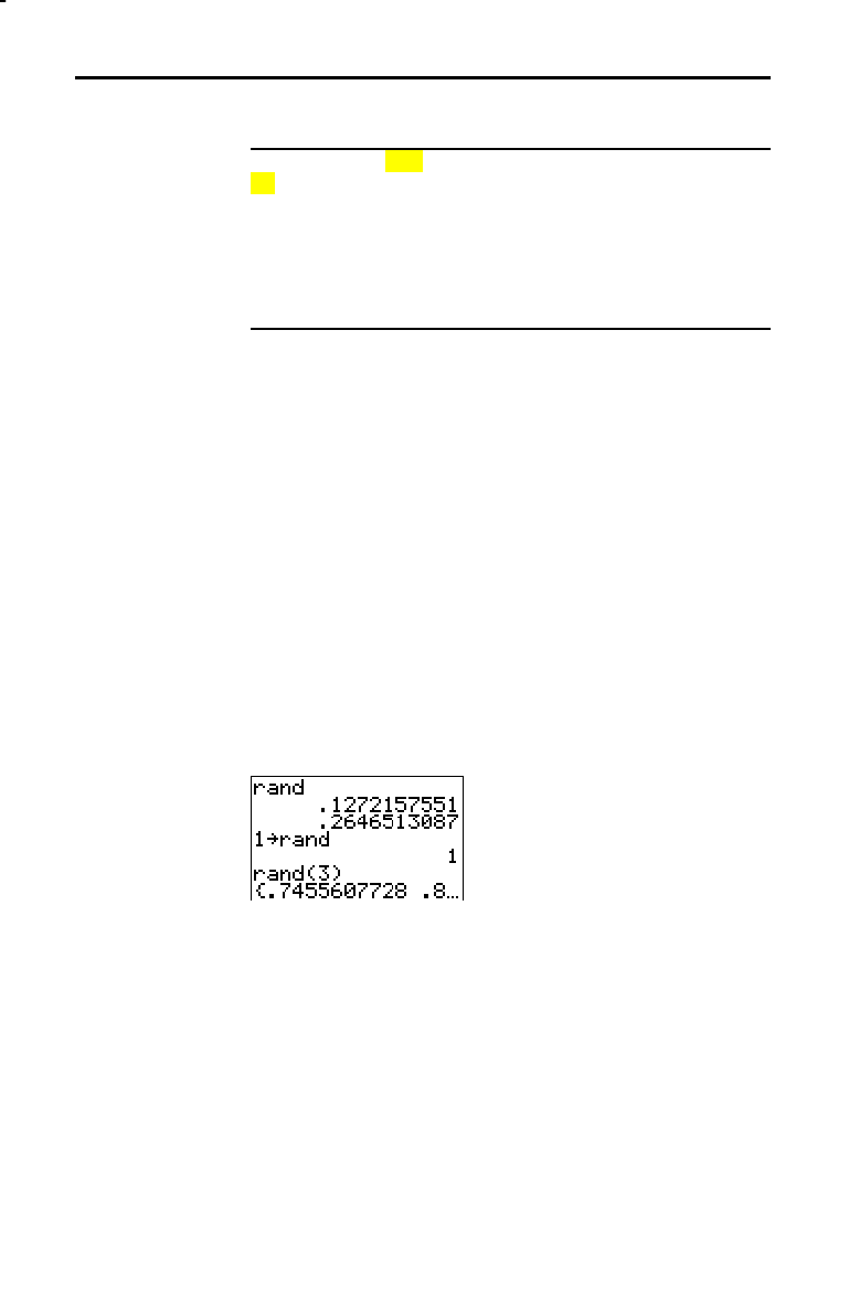
2-20 Math, Angle, and Test Operations
8302MATH.DOC TI-83 international English Bob Fedorisko Revised: 02/19/01 12:12 PM Printed: 02/19/01 2:27
PM Page 20 of 26
To display the
MATH PRB
menu, press
|
.
MATH NUM CPX PRB
1: rand
Random-number generator
2: nPr
Number of permutations
3: nCr
Number of combinations
4: !
Factorial
5: randInt(
Random-integer generator
6: randNorm(
Random # from Normal distribution
7: randBin(
Random # from Binomial distribution
rand (random number) generates and returns one or more
random numbers > 0 and < 1. To generate a list of random-
numbers, specify an integer > 1 for
numtrials
(number of
trials). The default for
numtrials
is 1.
rand[(
numtrials
)]
Tip:
To generate random numbers beyond the range of 0 to 1, you
can include
rand
in an expression. For example,
rand
ä
5
generates a
random number > 0 and < 5.
With each rand execution, the TI
-
83 generates the same
random-number sequence for a given seed value. The TI
-
83
factory-set seed value for
rand is 0. To generate a different
random-number sequence, store any nonzero seed value to
rand. To restore the factory-set seed value, store 0 to rand
or reset the defaults (Chapter 18).
Note:
The seed value also affects
randInt(
,
randNorm(
, and
randBin(
instructions (page 2
.
22).
MATH PRB (Probability) Operations
MATH PRB Menu
rand
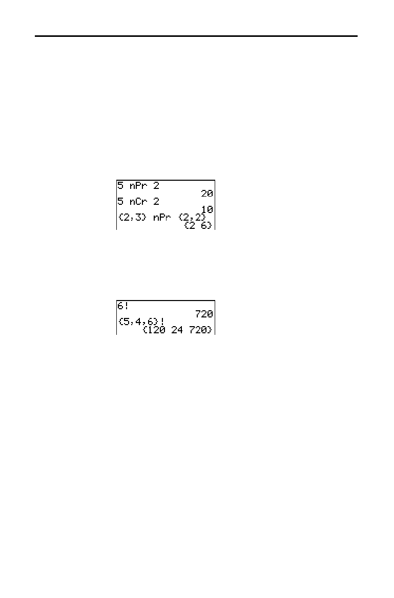
Math, Angle, and Test Operations 2-21
nPr (number of permutations) returns the number of
permutations of
items
taken
number
at a time.
items
and
number
must be nonnegative integers. Both
items
and
number
can be lists.
items
nPr
number
nCr (number of combinations) returns the number of
combinations of
items
taken
number
at a time.
items
and
number
must be nonnegative integers. Both
items
and
number
can be lists.
items
nCr
number
! (factorial) returns the factorial of either an integer or a
multiple of .5. For a list, it returns factorials for each
integer or multiple of .5.
value
must be
‚L
.5 and
69.
value
!
Note:
The factorial is computed recursively using the relationship
(n+1)! = n
ä
n!, until n is reduced to either 0 or
L
1/2. At that point, the
definition 0!=1 or the definition (
L
1
à
2)!=
‡p
is used to complete the
calculation. Hence:
n!=n
ä
(n
N
1)
ä
(n
N
2)
ä
...
ä
2
ä
1, if n is an integer
‚
0
n!= n
ä
(n
N
1)
ä
(n
N
2)
ä
...
ä
1
à
2
ä
‡p
, if n+1
à
2 is an integer
‚
0
n! is an error, if neither n nor n+1
à
2 is an integer
‚
0.
(The variable n equals
value
in the syntax description above.)
nPr,
nCr
! (Factorial)
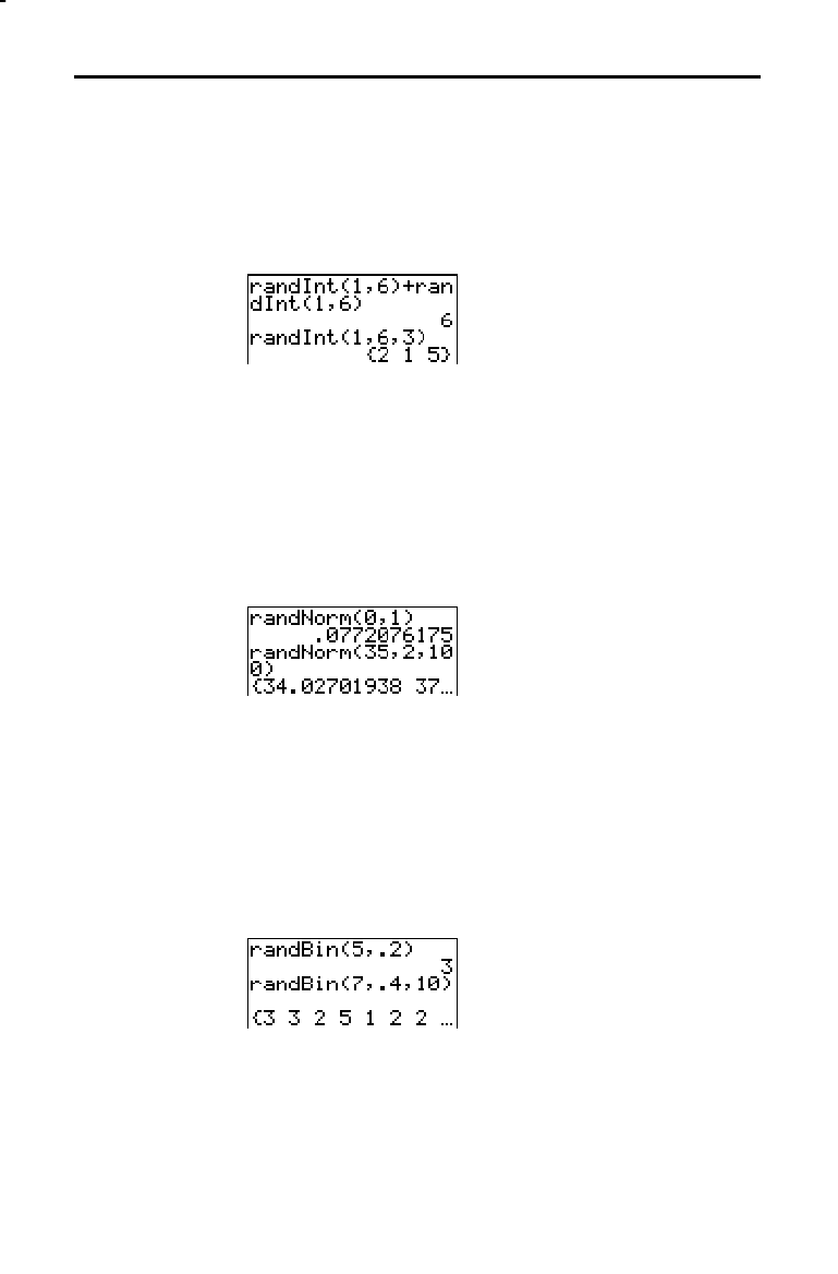
2-22 Math, Angle, and Test Operations
8302MATH.DOC TI-83 international English Bob Fedorisko Revised: 02/19/01 12:12 PM Printed: 02/19/01 2:27
PM Page 22 of 26
randInt( (random integer) generates and displays a random
integer within a range specified by
lower
and
upper
integer
bounds. To generate a list of random numbers, specify an
integer >1 for
numtrials
(number of trials); if not
specified, the default is 1.
randInt(
lower
,
upper
[
,
numtrials
]
)
randNorm( (random Normal) generates and displays a
random real number from a specified Normal distribution.
Each generated value could be any real number, but most
will be within the interval [
mN
3(
s
),
m
+3(
s
)]. To generate a
list of random numbers, specify an integer > 1 for
numtrials
(number of trials); if not specified, the default
is 1.
randNorm(
m
,
s
[,
numtrials
]
)
randBin( (random Binomial) generates and displays a
random integer from a specified Binomial distribution.
numtrials
(number of trials) must be
‚
1.
prob
(probability
of success) must be
‚
0 and
1. To generate a list of
random numbers, specify an integer > 1 for
numsimulations
(number of simulations); if not specified,
the default is 1.
randBin(
numtrials
,
prob
[
,
numsimulations
]
)
Note:
The seed value stored to
rand
also affects
randInt(
,
randNorm(
, and
randBin(
instructions (page 2
-
20).
randInt(
randNorm(
randBin(
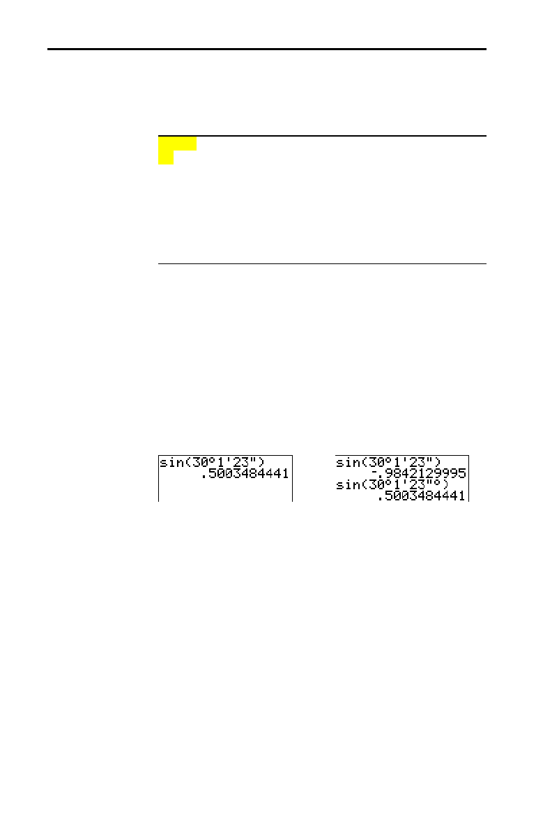
Math, Angle, and Test Operations 2-23
To display the
ANGLE
menu, press
y
[
ANGLE
]. The
ANGLE
menu displays angle indicators and instructions. The
Radian/Degree mode setting affects the TI
-
83’s
interpretation of
ANGLE
menu entries.
ANGLE
1:
¡
Degree notation
2: '
DMS minute notation
3:
r
Radian notation
4:
8
DMS
Displays as degree/minute/second
5: R
8
Pr(
Returns
r
, given
X
and
Y
6: R
8
P
q
(
Returns
q
, given
X
and
Y
7: P
8
Rx(
Returns
x
, given
R
and
q
8: P
8
Ry(
Returns
y
, given
R
and
q
DMS (degrees/minutes/seconds) entry notation comprises
the degree symbol (
¡
), the minute symbol ('), and the
second symbol (
").
degrees
must be a real number;
minutes
and
seconds
must be real numbers
‚
0.
degrees
¡
minutes
'
seconds
"
For example, enter for 30 degrees, 1 minute, 23 seconds. If
the angle mode is not set to
Degree, you must use
¡
so that
the TI
-
83 can interpret the argument as degrees, minutes,
and seconds.
Degree mode Radian mode
¡
(degree) designates an angle or list of angles as degrees,
regardless of the current angle mode setting. In
Radian
mode, you can use
¡
to convert degrees to radians.
value
¡
{
value1
,
value2
,
value3
,
value4
,...,
value n
}
¡
¡
also designates
degrees
(D) in DMS format.
' (minutes) designates
minutes
(M) in DMS format.
" (seconds) designates
seconds
(S) in DMS format.
Note:
"
is not on the
ANGLE
menu. To enter
"
, press
ƒ
[
ã
].
ANGLE Operations
ANGLE Menu
DMS Entry
Notation
¡
(Degree)
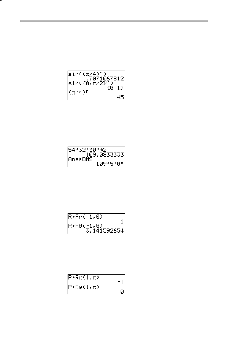
2-24 Math, Angle, and Test Operations
8302MATH.DOC TI-83 international English Bob Fedorisko Revised: 02/19/01 12:12 PM Printed: 02/19/01 2:27
PM Page 24 of 26
r
(radians) designates an angle or list of angles as radians,
regardless of the current angle mode setting. In
Degree
mode, you can use
r
to convert radians to degrees.
value
r
Degree mode
8
DMS
(degree/minute/second) displays
answer
in DMS
format (page 2
.
23). The mode setting must be
Degree for
answer
to be interpreted as degrees, minutes, and seconds.
8
DMS
is valid only at the end of a line.
answer
8
DMS
R
8
Pr( converts rectangular coordinates to polar
coordinates and returns
r. R
8
P
q
( converts rectangular
coordinates to polar coordinates and returns
q
.
x
and
y
can
be lists.
R
8
Pr(
x
,
y
), R
8
P
q
(
x
,
y
)
Note:
Radian
mode is set.
P
8
Rx(
converts polar coordinates to rectangular
coordinates and returns
x. P
8
Ry( converts polar
coordinates to rectangular coordinates and returns
y.
r
and
q
can be lists.
P
8
Rx(
r
,
q
), P
8
Ry(
r
,
q
)
Note:
Radian
mode is set.
r
(Radians)
8
DMS
R
8
Pr(,
R
8
P
q
(,
P
8
Rx(,
P
8
Ry(
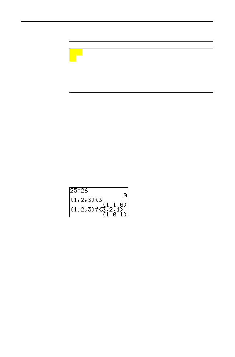
Math, Angle, and Test Operations 2-25
To display the
TEST
menu, press
y
[
TEST
].
This operator... Returns 1 (true) if...
TEST LOGIC
1:
=
Equal
2:
ƒ
Not equal to
3:
>
Greater than
4:
‚
Greater than or equal to
5:
<
Less than
6:
Less than or equal to
Relational operators compare
valueA
and
valueB
and
return
1
if the test is true or
0
if the test is false.
valueA
and
valueB
can be real numbers, expressions, or lists. For
=
and
ƒ
only,
valueA
and
valueB
also can be matrices or
complex numbers. If
valueA
and
valueB
are matrices, both
must have the same dimensions.
Relational operators are often used in programs to control
program flow and in graphing to control the graph of a
function over specific values.
valueA
=
valueB valueA
ƒ
valueB
valueA
>
valueB valueA
‚
valueB
valueA
<
valueB valueA
valueB
Relational operators are evaluated after mathematical
functions according to EOS rules (Chapter 1).
•
The expression
2+2=2+3
returns
0
. The TI
-
83 performs
the addition first because of EOS rules, and then it
compares 4 to 5.
•
The expression
2+(2=2)+3
returns
6
. The TI
-
83 performs
the relational test first because it is in parentheses, and
then it adds 2, 1, and 3.
TEST (Relational) Operations
TEST Menu
=,
ƒ
,
>,
‚
,
<,
Using Tests

2-26 Math, Angle, and Test Operations
8302MATH.DOC TI-83 international English Bob Fedorisko Revised: 02/19/01 12:12 PM Printed: 02/19/01 2:27
PM Page 26 of 26
To display the
TEST LOGIC
menu, press
y
ã
TESTä
~
.
This operator... Returns a 1 (true) if...
TEST LOGIC
1: and
Both values are nonzero (true).
2: or
At least one value is nonzero (true).
3: xor
Only one value is zero (false).
4: not(
The value is zero (false).
Boolean operators are often used in programs to control
program flow and in graphing to control the graph of the
function over specific values. Values are interpreted as
zero (false) or nonzero (true).
and
,
or
, and
xor
(exclusive or) return a value of
1
if an
expression is true or
0
if an expression is false, according
to the table below.
valueA
and
valueB
can be real
numbers, expressions, or lists.
valueA
and
valueB
valueA
or
valueB
valueA
xor
valueB
valueA valueB and or xor
ƒ
0
ƒ
0 returns
110
ƒ
0 0 returns
011
0
ƒ
0 returns
011
0 0 returns
000
not(
returns
1
if
value
(which can be an expression) is
0
.
not(
value
)
Boolean logic is often used with relational tests. In the
following program, the instructions store
4
into
C
.
TEST LOGIC (Boolean) Operations
TEST LOGIC
Menu
Boolean
Operators
and,
or,
xor
not(
Using Boolean
Operations
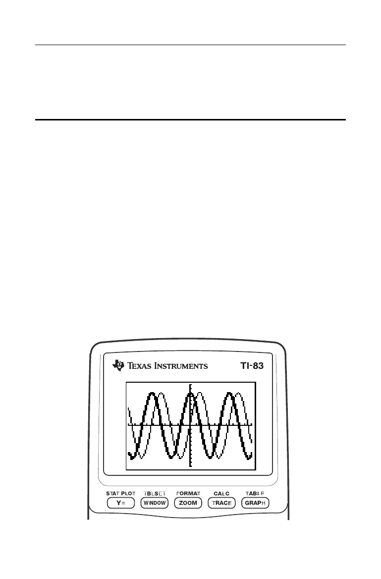
Function Graphing 3-1
8303FUNC.DOC TI-83 international English Bob Fedorisko Revised: 02/19/01 12:16 PM Printed: 02/19/01 1:50
PM Page 1 of 28
3
Function
Graphin
g
Getting Started: Graphing a Circle
.......................
3-2
Defining Graphs
.........................................
3-3
Setting the Graph Modes
.................................
3-4
Defining Functions
......................................
3-5
Selecting and Deselecting Functions
.....................
3-7
Setting Graph Styles for Functions
.......................
3-9
Setting the Viewing Window Variables
...................
3-11
Setting the Graph Format
................................
3-13
Displaying Graphs
.......................................
3-15
Exploring Graphs with the Free-Moving Cursor
..........
3-17
Exploring Graphs with
TRACE
...........................
3-18
Exploring Graphs with the
ZOOM
Instructions
...........
3-20
Using
ZOOM MEMORY
..................................
3-23
Using the
CALC
(Calculate) Operations
..................
3-25
Contents
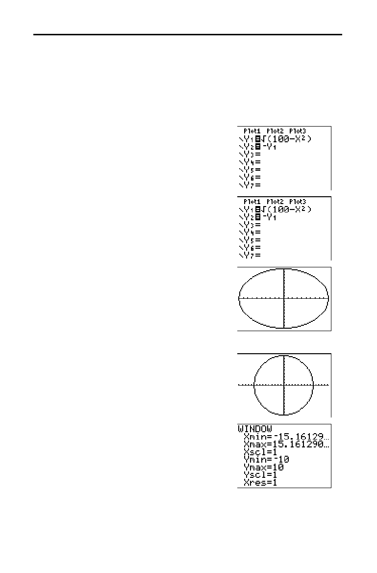
3-2 Function Graphing
8303FUNC.DOC TI-83 international English Bob Fedorisko Revised: 02/19/01 12:16 PM Printed: 02/19/01 1:35
PM Page 2 of 28
8303FUNC.DOC TI-83 international English Bob Fedorisko Revised: 02/19/01 12:16 PM Printed: 02/19/01 1:35
PM Page 2 of 28
Getting Started is a fast-paced introduction. Read the chapter for details.
Graph a circle of radius 10, centered on the origin in the standard viewing
window. To graph this circle, you must enter separate formulas for the upper
and lower portions of the circle. Then use
ZSquare (zoom square) to adjust the
display and make the functions appear as a circle.
1. In
Func mode, press
o
to display the
Y=
editor. Press
y
ã
‡
ä
100
¹
„
¡
¤
Í
to enter the expression Y=
‡
(100
N
X
2
),
which defines the top half of the circle.
The expression Y=
L‡
(100
N
X
2
) defines the
bottom half of the circle. On the TI
-
83, you
can define one function in terms of another.
To define
Y
2
=
L
Y
1
, press
Ì
to enter the
negation sign. Press
~
to display the
VARS Y
.
VARS
menu. Then press
Í
to
select
1:Function. The
FUNCTION
secondary
menu is displayed. Press
1 to select 1:Y
1
.
2. Press
q
6 to select 6:ZStandard. This is a
quick way to reset the window variables to
the standard values. It also graphs the
functions; you do not need to press
s
.
Notice that the functions appear as an
ellipse in the standard viewing window.
3. To adjust the display so that each pixel
represents an equal width and height, press
q
5 to select 5:ZSquare. The functions
are replotted and now appear as a circle on
the display.
4. To see the ZSquare window variables, press
p
and notice the new values for
Xmin,
Xmax, Ymin, and Ymax.
Getting Started: Graphing a Circle

Function Graphing 3-3
8303FUNC.DOC TI-83 international English Bob Fedorisko Revised: 02/19/01 12:16 PM Printed: 02/19/01 1:35
PM Page 3 of 28
Chapter 3 specifically describes function graphing, but the
steps shown here are similar for each TI
-
83 graphing
mode. Chapters 4, 5, and 6 describe aspects that are unique
to parametric graphing, polar graphing, and sequence
graphing.
To define a graph in any graphing mode, follow these
steps. Some steps are not always necessary.
1. Press
z
and set the appropriate graph mode
(page 3
.
4).
2. Press
o
and enter, edit, or select one or more functions
in the
Y=
editor (page 3
.
5 and 3
.
7).
3. Deselect stat plots, if necessary (page 3
.
7).
4. Set the graph style for each function (page 3
.
9).
5. Press
p
and define the viewing window variables
(page 3
.
11).
6. Press
y
[
FORMAT
] and select the graph format settings
(page 3
.
13).
After you have defined a graph, press
s
to display it.
Explore the behavior of the function or functions using the
TI
-
83 tools described in this chapter.
You can store the elements that define the current graph to
any of 10 graph database variables (
GDB1 through GDB9,
and
GDB0; Chapter 8). To recreate the current graph later,
simply recall the graph database to which you stored the
original graph.
These types of information are stored in a
GDB.
•
Y=
functions
•
Graph style settings
•
Window settings
•
Format settings
You can store a picture of the current graph display to any
of 10 graph picture variables (
Pic1 through Pic9, and Pic0;
Chapter 8). Then you can superimpose one or more stored
pictures onto the current graph.
Defining Graphs
TI-83—Graphing
Mode Similarities
Defining a Graph
Displaying and
Exploring a
Graph
Saving a Graph
for Later Use
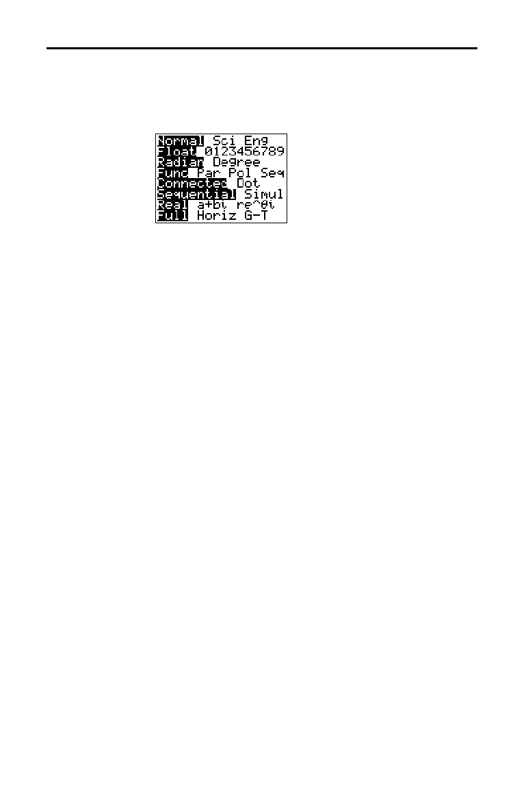
3-4 Function Graphing
8303FUNC.DOC TI-83 international English Bob Fedorisko Revised: 02/19/01 12:16 PM Printed: 02/19/01 1:35
PM Page 4 of 28
8303FUNC.DOC TI-83 international English Bob Fedorisko Revised: 02/19/01 12:16 PM Printed: 02/19/01 1:35
PM Page 4 of 28
To display the mode screen, press
z
. The default
settings are highlighted below. To graph functions, you
must select
Func mode before you enter values for the
window variables and before you enter the functions.
The TI
-
83 has four graphing modes.
•
Func (function graphing)
•
Par (parametric graphing; Chapter 4)
•
Pol (polar graphing; Chapter 5)
•
Seq (sequence graphing; Chapter 6)
Other mode settings affect graphing results. Chapter 1
describes each mode setting.
•
Float or 0123456789 (fixed) decimal mode affects
displayed graph coordinates.
•
Radian or Degree angle mode affects interpretation of
some functions.
•
Connected or Dot plotting mode affects plotting of
selected functions.
•
Sequential or Simul graphing-order mode affects
function plotting when more than one function is
selected.
To set the graphing mode and other modes from a
program, begin on a blank line in the program editor and
follow these steps.
1. Press
z
to display the mode settings.
2. Press
†
,
~
,
|
, and
}
to place the cursor on the mode
that you want to select.
3. Press
Í
to paste the mode name to the cursor
location.
The mode is changed when the program is executed.
Setting the Graph Modes
Checking and
Changing the
Graphing Mode
Setting Modes
from a Program
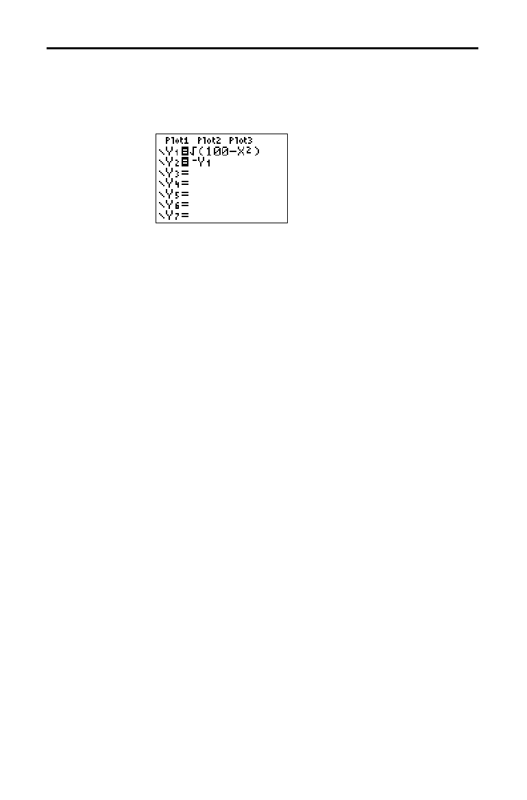
Function Graphing 3-5
8303FUNC.DOC TI-83 international English Bob Fedorisko Revised: 02/19/01 12:16 PM Printed: 02/19/01 1:35
PM Page 5 of 28
To display the
Y=
editor, press
o
. You can store up to 10
functions to the function variables
Y
1
through Y
9
, and Y
0
.
You can graph one or more defined functions at once. In
this example, functions
Y
1
and Y
2
are defined and selected.
To define or edit a function, follow these steps.
1. Press
o
to display the
Y=
editor.
2. Press
†
to move the cursor to the function you want to
define or edit. To erase a function, press
‘
.
3. Enter or edit the expression to define the function.
•
You may use functions and variables (including
matrices and lists) in the expression. When the
expression evaluates to a nonreal number, the value
is not plotted; no error is returned.
•
The independent variable in the function is
X. Func
mode defines
„
as X. To enter X, press
„
or press
ƒ
[
X
].
•
When you enter the first character, the
= is
highlighted, indicating that the function is selected.
As you enter the expression, it is stored to the variable
Y
n
as a user-defined function in the
Y=
editor.
4. Press
Í
or
†
to move the cursor to the next
function.
Defining Functions
Displaying
Functions in the
Y= Editor
Defining or
Editing a
Function
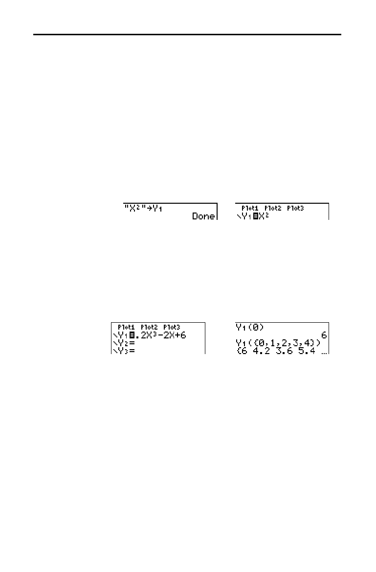
3-6 Function Graphing
8303FUNC.DOC TI-83 international English Bob Fedorisko Revised: 02/19/01 12:16 PM Printed: 02/19/01 1:35
PM Page 6 of 28
8303FUNC.DOC TI-83 international English Bob Fedorisko Revised: 02/19/01 12:16 PM Printed: 02/19/01 1:35
PM Page 6 of 28
To define a function from the home screen or a program,
begin on a blank line and follow these steps.
1. Press
ƒ
[
ã
], enter the expression, and then press
ƒ
[
ã
] again.
2. Press
¿
.
3. Press
~
1 to select 1:Function from the
VARS Y
.
VARS
menu.
4. Select the function name, which pastes the name to the
cursor location on the home screen or program editor.
5. Press
Í
to complete the instruction.
"
expression
"
!
Y
n
When the instruction is executed, the TI
-
83 stores the
expression to the designated variable
Y
n
, selects the
function, and displays the message
Done.
You can calculate the value of a
Y=
function Y
n
at a
specified
value
of
X. A list of
values
returns a list.
Y
n
(
value
)
Y
n
({
value1
,
value2
,
value3
,
. . .
,
value n
})
Defining a
Function from
the Home Screen
or a Program
Evaluating Y=
Functions in
Expressions
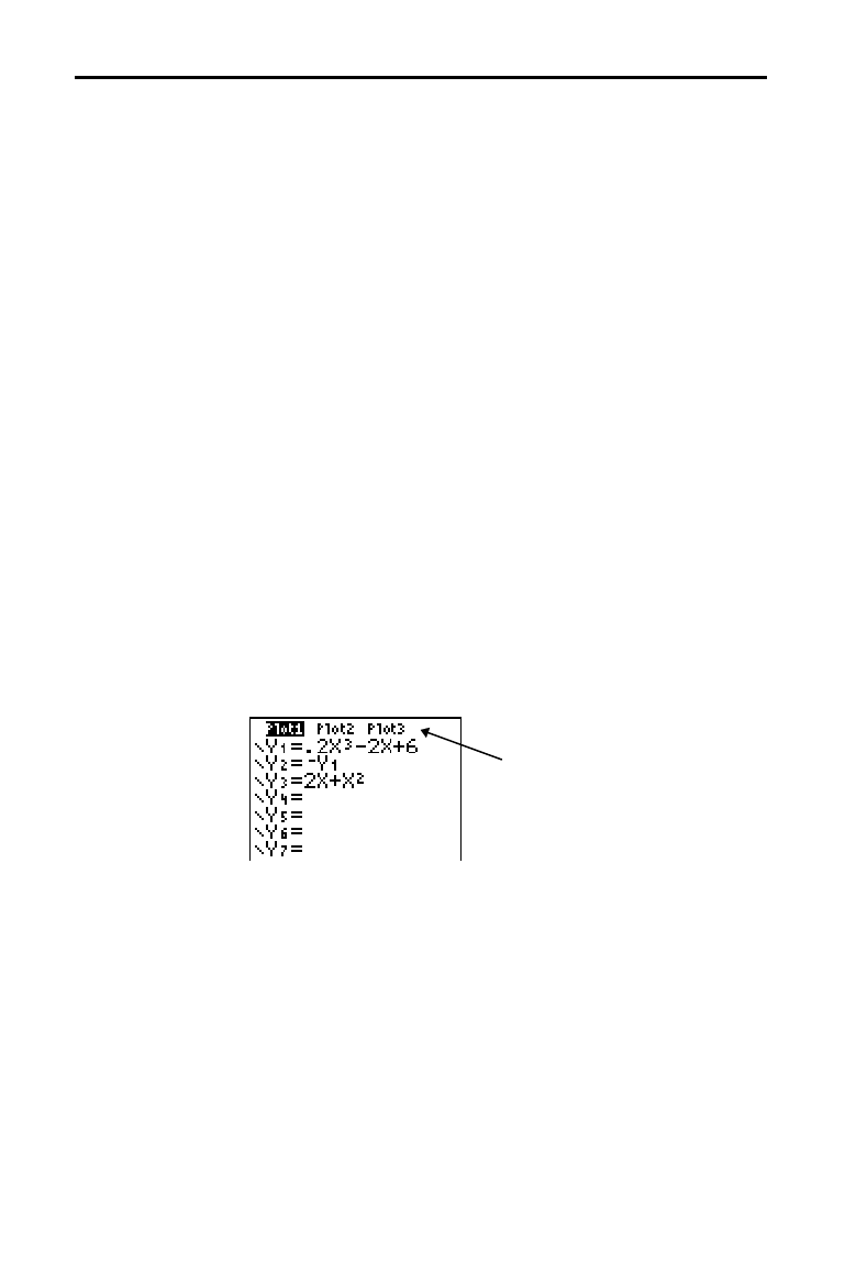
Function Graphing 3-7
8303FUNC.DOC TI-83 international English Bob Fedorisko Revised: 02/19/01 12:16 PM Printed: 02/19/01 1:35
PM Page 7 of 28
You can select and deselect (turn on and turn off) a
function in the
Y=
editor. A function is selected when the =
sign is highlighted. The TI
-
83 graphs only the selected
functions. You can select any or all functions
Y
1
through
Y
9
, and Y
0
.
To select or deselect a function in the
Y=
editor, follow
these steps.
1. Press
o
to display the
Y=
editor.
2. Move the cursor to the function you want to select or
deselect.
3. Press
|
to place the cursor on the function’s
= sign.
4. Press
Í
to change the selection status.
When you enter or edit a function, it is selected
automatically. When you clear a function, it is deselected.
To view and change the on/off status of a stat plot in the
Y=
editor, use Plot1 Plot2 Plot3 (the top line of the
Y=
editor). When a plot is on, its name is highlighted on this
line.
To change the on/off status of a stat plot from the
Y=
editor, press
}
and
~
to place the cursor on Plot1,
Plot2, or Plot3, and then press
Í
.
Selecting and Deselecting Functions
Selecting and
Deselecting a
Function
Turning On or
Turning Off a Stat
Plot in the Y=
Editor
Plot1
is turned on.
Plot2
and
Plot3
are turned off.
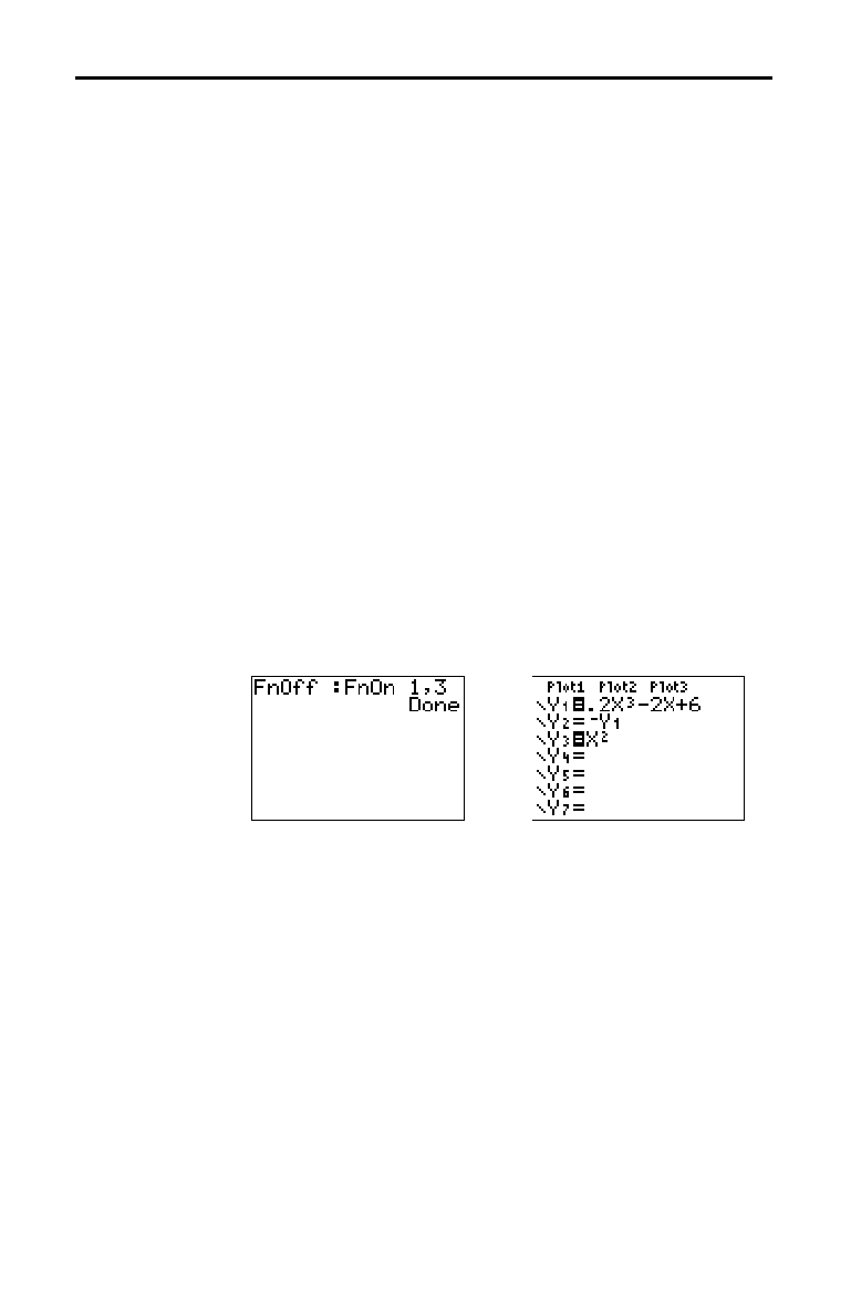
3-8 Function Graphing
8303FUNC.DOC TI-83 international English Bob Fedorisko Revised: 02/19/01 12:16 PM Printed: 02/19/01 1:35
PM Page 8 of 28
8303FUNC.DOC TI-83 international English Bob Fedorisko Revised: 02/19/01 12:16 PM Printed: 02/19/01 1:35
PM Page 8 of 28
To select or deselect a function from the home screen or a
program, begin on a blank line and follow these steps.
1. Press
~
to display the
VARS Y
.
VARS
menu.
2. Select
4:On/Off to display the
ON/OFF
secondary menu.
3. Select
1:FnOn to turn on one or more functions or
2:FnOff to turn off one or more functions. The
instruction you select is copied to the cursor location.
4. Enter the number (
1 through 9, or 0; not the variable
Y
n
) of each function you want to turn on or turn off.
•
If you enter two or more numbers, separate them
with commas.
•
To turn on or turn off all functions, do not enter a
number after
FnOn or FnOff.
FnOn[
function#
,
function#
, . . .,
function n
]
FnOff[
function#
,
function#
, . . .,
function n
]
5. Press
Í
. When the instruction is executed, the
status of each function in the current mode is set and
Done is displayed.
For example, in
Func mode, FnOff :FnOn 1,3 turns off all
functions in the
Y=
editor, and then turns on Y
1
and Y
3
.
Selecting and
Deselecting
Functions from
the Home Screen
or a Program
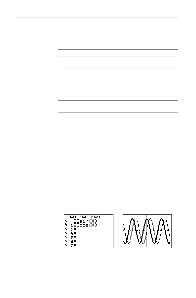
Function Graphing 3-9
8303FUNC.DOC TI-83 international English Bob Fedorisko Revised: 02/19/01 12:16 PM Printed: 02/19/01 1:35
PM Page 9 of 28
This table describes the graph styles available for function
graphing. Use the styles to visually differentiate functions
to be graphed together. For example, you can set
Y
1
as a
solid line,
Y
2
as a dotted line, and Y
3
as a thick line.
Icon Style Description
ç
Line A solid line connects plotted points; this is
the default in
Connected mode
è
Thick A thick solid line connects plotted points
é
Above Shading covers the area a*bove the graph
ê
Below Shading covers the area below the graph
ë
Path A circular cursor traces the leadin
g
ed
g
e of
the graph and draws a path
ì
Animate A circular cursor traces the leadin
g
ed
g
e of
the graph without drawing a path
í
Dot A small dot represents each plotted point;
this is the default in
Dot mode
Note:
Some graph styles are not available in all graphing modes.
Chapters 4, 5, and 6 list the styles for
Par
,
Pol
, and
Seq
modes.
To set the graph style for a function, follow these steps.
1. Press
o
to display the
Y=
editor.
2. Press
†
and
}
to move the cursor to the function.
3. Press
|
|
to move the cursor left, past the
= sign, to
the graph style icon in the first column. The insert
cursor is displayed. (Steps 2 and 3 are interchangeable.)
4. Press
Í
repeatedly to rotate through the graph
styles. The seven styles rotate in the same order in
which they are listed in the table above.
5. Press
~
,
}
, or
†
when you have selected a style.
Setting Graph Styles for Functions
Graph Style
Icons in the Y=
Editor
Setting the Graph
Style
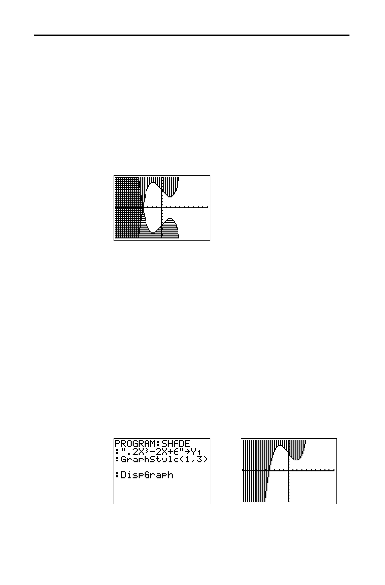
3-10 Function Graphing
8303FUNC.DOC TI-83 international English Bob Fedorisko Revised: 02/19/01 12:16 PM Printed: 02/19/01 1:35
PM Page 10 of 28
8303FUNC.DOC TI-83 international English Bob Fedorisko Revised: 02/19/01 12:16 PM Printed: 02/19/01 1:35
PM Page 10 of 28
When you select
é
or
ê
for two or more functions, the
TI
-
83 rotates through four shading patterns.
•
Vertical lines shade the first function with a
é
or
ê
graph style.
•
Horizontal lines shade the second.
•
Negatively sloping diagonal lines shade the third.
•
Positively sloping diagonal lines shade the fourth.
•
The rotation returns to vertical lines for the fifth
é
or
ê
function, repeating the order described above.
When shaded areas intersect, the patterns overlap.
Note:
When
é
or
ê
is selected for a Y= function that graphs a family of
curves, such as
Y1={1,2,3}X
, the four shading patterns rotate for
each member of the family of curves.
To set the graph style from a program, select
H:GraphStyle(
from the
PRGM CTL
menu. To display this menu, press
while in the program editor.
function#
is the number
of the
Y=
function name in the current graphing mode.
graphstyle#
is an integer from
1
to
7
that corresponds to
the graph style, as shown below.
1
=
ç
(line)
2
=
è
(thick)
3
=
é
(above)
4
=
ê
(below)
5
=
ë
(path)
6
=
ì
(animate)
7
=
í
(dot)
GraphStyle(
function#
,
graphstyle#
)
For example, when this program is executed in
Func
mode,
GraphStyle(1,3)
sets
Y
1
to
é
(above).
Shading Above
and Below
Setting a Graph
Style from a
Program
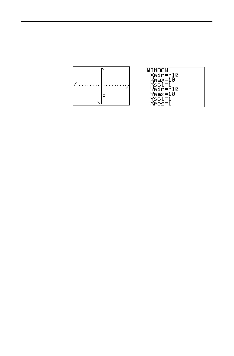
Function Graphing 3-11
8303FUNC.DOC TI-83 international English Bob Fedorisko Revised: 02/19/01 12:16 PM Printed: 02/19/01 1:35
PM Page 11 of 28
The viewing window is the portion of the coordinate plane
defined by
Xmin, Xmax, Ymin, and Ymax. Xscl (X scale)
defines the distance between tick marks on the x-axis.
Yscl
(Y scale) defines the distance between tick marks on the
y-axis. To turn off tick marks, set
Xscl=0 and Yscl=0.
Xmax
Ymin
Ymax
Xscl
Yscl
Xmin
To display the current window variable values, press
p
. The window editor above and to the right shows
the default values in
Func graphing mode and Radian angle
mode. The window variables differ from one graphing
mode to another.
Xres sets pixel resolution (1 through 8) for function graphs
only. The default is
1.
•
At
Xres=1, functions are evaluated and graphed at each
pixel on the x-axis.
•
At
Xres=8, functions are evaluated and graphed at every
eighth pixel along the x-axis.
Tip:
Small
Xres
values improve graph resolution but may cause the
TI
-
83 to draw graphs more slowly.
To change a window variable value from the window
editor, follow these steps.
1. Press
†
or
}
to move the cursor to the window
variable you want to change.
2. Edit the value, which can be an expression.
•
Enter a new value, which clears the original value.
•
Move the cursor to a specific digit, and then edit it.
3. Press
Í
,
†
, or
}
. If you entered an expression, the
TI
-
83 evaluates it. The new value is stored.
Note:
Xmin
<
Xmax
and
Ymin
<
Ymax
must be true in order to graph.
Setting the Viewing Window Variables
The TI-83 Viewing
Window
Displaying the
Window
Variables
Changing a
Window Variable
Value
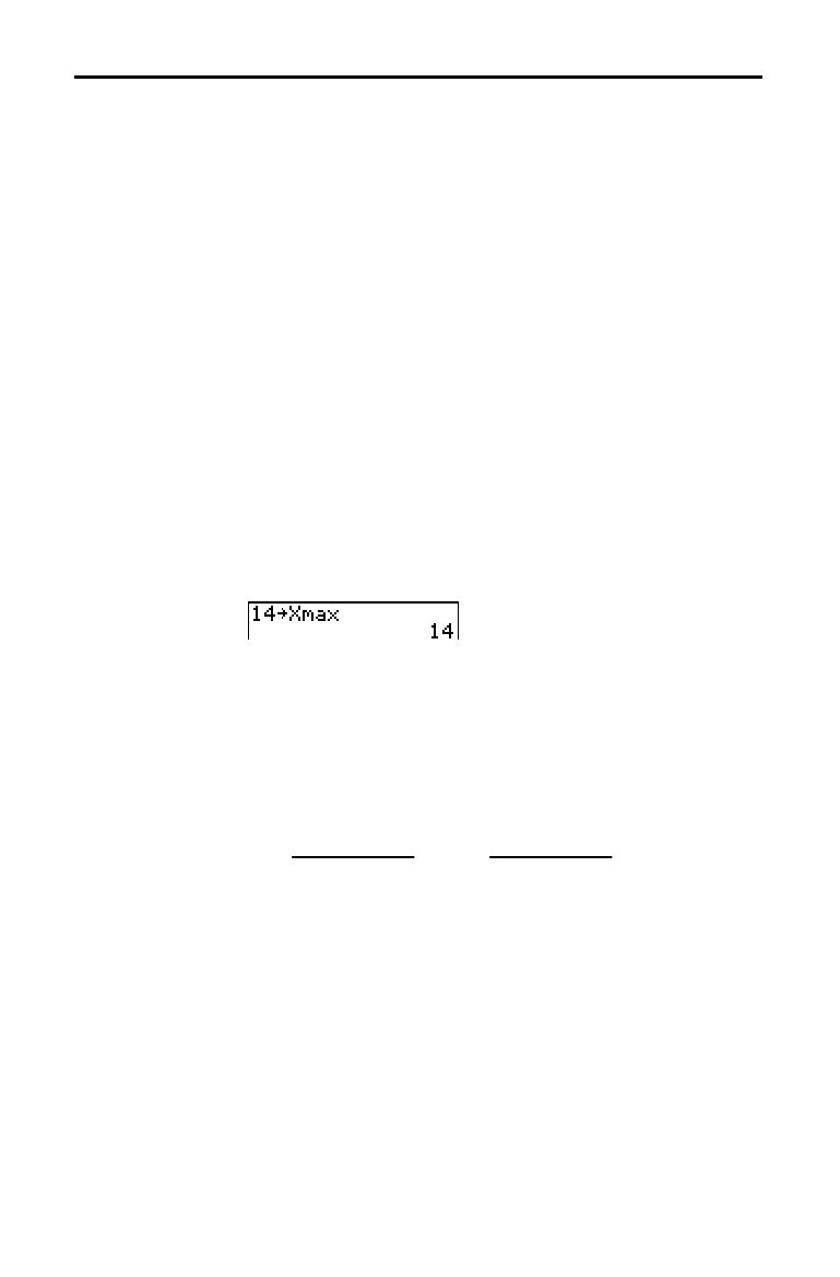
3-12 Function Graphing
8303FUNC.DOC TI-83 international English Bob Fedorisko Revised: 02/19/01 12:16 PM Printed: 02/19/01 1:35
PM Page 12 of 28
8303FUNC.DOC TI-83 international English Bob Fedorisko Revised: 02/19/01 12:16 PM Printed: 02/19/01 1:35
PM Page 12 of 28
To store a value, which can be an expression, to a window
variable, begin on a blank line and follow these steps.
1. Enter the value you want to store.
2. Press
¿
.
3. Press
to display the
VARS
menu.
4. Select
1:Window to display the Func window variables
(
X/Y
secondary menu).
•
Press
~
to display the
Par and Pol window variables
(
T/
q
secondary menu).
•
Press
~
~
to display the
Seq window variables
(
U/V/W
secondary menu).
5. Select the window variable to which you want to store a
value. The name of the variable is pasted to the current
cursor location.
6. Press
Í
to complete the instruction.
When the instruction is executed, the TI
-
83 stores the
value to the window variable and displays the value.
The variables
@
X
and
@
Y
(items 8 and 9 on the
VARS
(1:Window)
X/Y
secondary menu) define the distance from
the center of one pixel to the center of any adjacent pixel
on a graph (graphing accuracy).
@
X and
@
Y are calculated
from
Xmin, Xmax, Ymin, and Ymax when you display a
graph.
@
X
=
(Xmax
N
Xmin)
94
@
Y =
(Ymax
N
Ymin)
62
You can store values to
@
X
and
@
Y
. If you do, Xmax and
Ymax are calculated from
@
X
, Xmin,
@
Y
, and Ymin.
Storing to a
Window Variable
from the Home
Screen or a
Program
@
X and
@
Y

Function Graphing 3-13
8303FUNC.DOC TI-83 international English Bob Fedorisko Revised: 02/19/01 12:16 PM Printed: 02/19/01 1:35
PM Page 13 of 28
To display the format settings, press
y
[
FORMAT
]. The
default settings are highlighted below.
RectGC PolarGC
Sets cursor coordinates.
CoordOn CoordOff
Sets coordinates display on or off.
GridOff GridOn
Sets grid off or on.
AxesOn AxesOff
Sets axes on or off.
LabelOff LabelOn
Sets axes label off or on.
ExprOn ExprOff
Sets expression display on or off.
Format settings define a graph’s appearance on the display.
Format settings apply to all graphing modes.
Seq graphing
mode has an additional mode setting (Chapter 6).
To change a format setting, follow these steps.
1. Press
†
,
~
,
}
, and
|
as necessary to move the cursor
to the setting you want to select.
2. Press
Í
to select the highlighted setting.
RectGC (rectangular graphing coordinates) displays the
cursor location as rectangular coordinates
X and Y.
PolarGC (polar graphing coordinates) displays the cursor
location as polar coordinates
R and
q
.
The
RectGC/PolarGC setting determines which variables
are updated when you plot the graph, move the free-
moving cursor, or trace.
•
RectGC updates X and Y; if CoordOn format is selected,
X and Y are displayed.
•
PolarGC updates X, Y, R, and
q
; if CoordOn format is
selected, R and
q
are displayed.
Setting the Graph Format
Displaying the
Format Settings
Changing a
Format Setting
RectGC, PolarGC

3-14 Function Graphing
8303FUNC.DOC TI-83 international English Bob Fedorisko Revised: 02/19/01 12:16 PM Printed: 02/19/01 1:35
PM Page 14 of 28
8303FUNC.DOC TI-83 international English Bob Fedorisko Revised: 02/19/01 12:16 PM Printed: 02/19/01 1:35
PM Page 14 of 28
CoordOn (coordinates on) displays the cursor coordinates
at the bottom of the graph. If
ExprOff format is selected,
the function number is displayed in the top-right corner.
CoordOff (coordinates off) does not display the function
number or coordinates.
Grid points cover the viewing window in rows that
correspond to the tick marks (page 3
.
11) on each axis.
GridOff does not display grid points.
GridOn displays grid points.
AxesOn displays the axes.
AxesOff does not display the axes.
This overrides the
LabelOff/LabelOn format setting.
LabelOff and LabelOn determine whether to display labels
for the axes (
X and Y), if AxesOn format is also selected.
ExprOn and ExprOff determine whether to display the
Y=
expression when the trace cursor is active. This format
setting also applies to stat plots.
When
ExprOn is selected, the expression is displayed in the
top-left corner of the graph screen.
When
ExprOff and CoordOn both are selected, the number
in the top-right corner specifies which function is being
traced.
CoordOn,
CoordOff
GridOff, GridOn
AxesOn, AxesOff
LabelOff,
LabelOn
ExprOn, ExprOff

Function Graphing 3-15
8303FUNC.DOC TI-83 international English Bob Fedorisko Revised: 02/19/01 12:16 PM Printed: 02/19/01 1:35
PM Page 15 of 28
To display the graph of the selected function or functions,
press
s
.
TRACE
,
ZOOM
instructions, and
CALC
operations display the graph automatically. As the TI
-
83
plots the graph, the busy indicator is on. As the graph is
plotted,
X and Y are updated.
While plotting a graph, you can pause or stop graphing.
•
Press
Í
to pause; then press
Í
to resume.
•
Press
É
to stop; then press
s
to redraw.
Smart Graph is a TI
-
83 feature that redisplays the last
graph immediately when you press
s
, but only if all
graphing factors that would cause replotting have
remained the same since the graph was last displayed.
If you performed any of these actions since the graph was
last displayed, the TI
-
83 will replot the graph based on new
values when you press
s
.
•
Changed a mode setting that affects graphs
•
Changed a function in the current picture
•
Selected or deselected a function or stat plot
•
Changed the value of a variable in a selected function
•
Changed a window variable or graph format setting
•
Cleared drawings by selecting
ClrDraw
•
Changed a stat plot definition
Displaying Graphs
Displaying a New
Graph
Pausing or
Stopping a Graph
Smart Graph
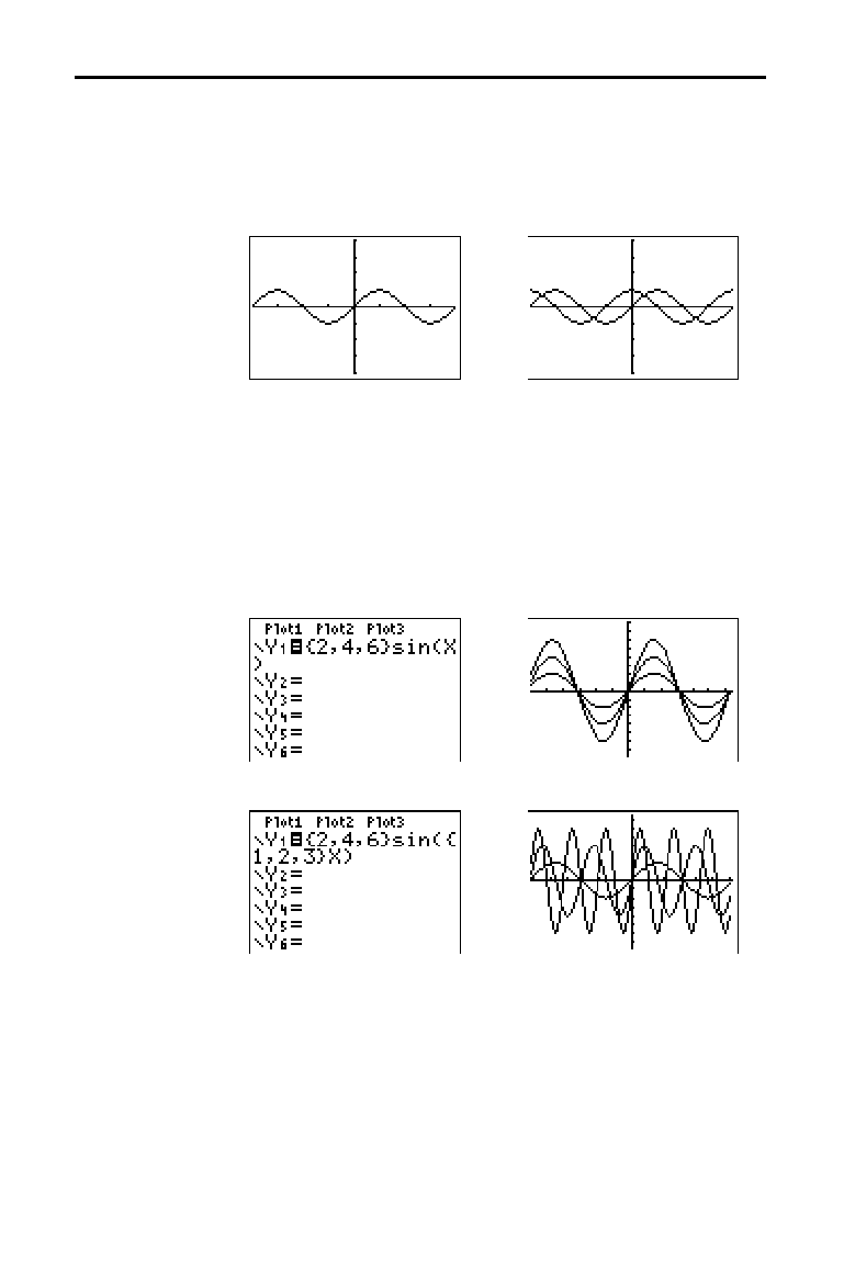
3-16 Function Graphing
8303FUNC.DOC TI-83 international English Bob Fedorisko Revised: 02/19/01 12:16 PM Printed: 02/19/01 1:35
PM Page 16 of 28
8303FUNC.DOC TI-83 international English Bob Fedorisko Revised: 02/19/01 12:16 PM Printed: 02/19/01 1:35
PM Page 16 of 28
On the TI
-
83, you can graph one or more new functions
without replotting existing functions. For example, store
sin(X) to Y
1
in the
Y=
editor and press
s
. Then store
cos(X) to Y
2
and press
s
again. The function Y
2
is
graphed on top of
Y
1
, the original function.
If you enter a list (Chapter 11) as an element in an
expression, the TI
-
83 plots the function for each value in
the list, thereby graphing a family of curves. In
Simul
graphing-order mode, it graphs all functions sequentially
for the first element in each list, and then for the second,
and so on.
{2,4,6}sin(X) graphs three functions: 2 sin(X), 4 sin(X), and
6 sin(X).
{2,4,6}sin({1,2,3}X) graphs 2 sin(X), 4 sin(2X), and 6 sin(3X).
Note:
When using more than one list, the lists must have the same
dimensions.
Overlaying
Functions on a
Graph
Graphing a
Family of Curves
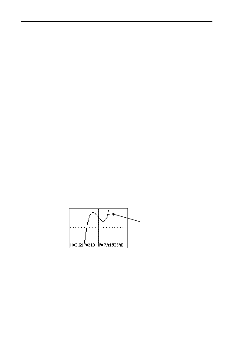
Function Graphing 3-17
8303FUNC.DOC TI-83 international English Bob Fedorisko Revised: 02/19/01 12:16 PM Printed: 02/19/01 1:35
PM Page 17 of 28
When a graph is displayed, press
|
,
~
,
}
, or
†
to move
the cursor around the graph. When you first display the
graph, no cursor is visible. When you press
|
,
~
,
}
, or
†
,
the cursor moves from the center of the viewing window.
As you move the cursor around the graph, the coordinate
values of the cursor location are displayed at the bottom of
the screen if
CoordOn format is selected. The Float/Fix
decimal mode setting determines the number of decimal
digits displayed for the coordinate values.
To display the graph with no cursor and no coordinate
values, press
‘
or
Í
. When you press
|
,
~
,
}
, or
†
, the cursor moves from the same position.
The free-moving cursor moves from pixel to pixel on the
screen. When you move the cursor to a pixel that appears
to be on the function, the cursor may be near, but not
actually on, the function. The coordinate value displayed at
the bottom of the screen actually may not be a point on the
function. To move the cursor along a function, use
r
(page 3
.
18).
The coordinate values displayed as you move the cursor
approximate actual math coordinates, *accurate to within
the width and height of the pixel. As
Xmin, Xmax, Ymin, and
Ymax get closer together (as in a ZoomIn) graphing
accuracy increases, and the coordinate values more closely
approximate the math coordinates.
Exploring Graphs with the Free-Moving Cursor
Free-Moving
Cursor
Graphing
Accuracy
Free-moving cursor “on” the curve
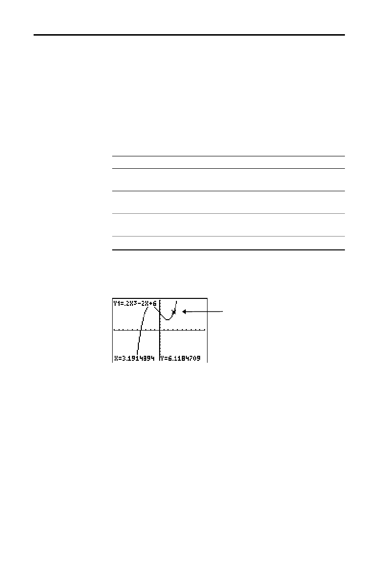
3-18 Function Graphing
8303FUNC.DOC TI-83 international English Bob Fedorisko Revised: 02/19/01 12:16 PM Printed: 02/19/01 1:35
PM Page 18 of 28
8303FUNC.DOC TI-83 international English Bob Fedorisko Revised: 02/19/01 12:16 PM Printed: 02/19/01 1:35
PM Page 18 of 28
Use
TRACE
to move the cursor from one plotted point to
the next along a function. To begin a trace, press
r
. If
the graph is not displayed already, press
r
to display
it. The trace cursor is on the first selected function in the
Y=
editor, at the middle X value on the screen. The cursor
coordinates are displayed at the bottom of the screen if
CoordOn format is selected. The
Y=
expression is displayed
in the top-left corner of the screen, if
ExprOn format is
selected.
To move the TRACE cursor . . . do this:
. . . to the previous or next plotted
point,
press
|
or
~
.
. . . five plotted points on a function
(Xres affects this),
press
y
|
or
y
~
.
. . . to any valid X value on a function, enter a value, and
then press
Í
.
. . . from one function to another, press
}
or
†
.
When the trace cursor moves along a function, the
Y value
is calculated from the
X value; that is, Y=Y
n
(X). If the
function is undefined at an
X value, the Y value is blank.
If you move the trace cursor beyond the top or bottom of
the screen, the coordinate values at the bottom of the
screen continue to change appropriately.
To move the trace cursor from function to function, press
†
and
}
. The cursor follows the order of the selected
functions in the
Y=
editor. The trace cursor moves to each
function at the same
X value. If ExprOn format is selected,
the expression is updated.
Exploring Graphs with TRACE
Beginning a
Trace
Moving the Trace
Cursor
Moving the Trace
Cursor from
Function to
Function
Trace cursor on the curve
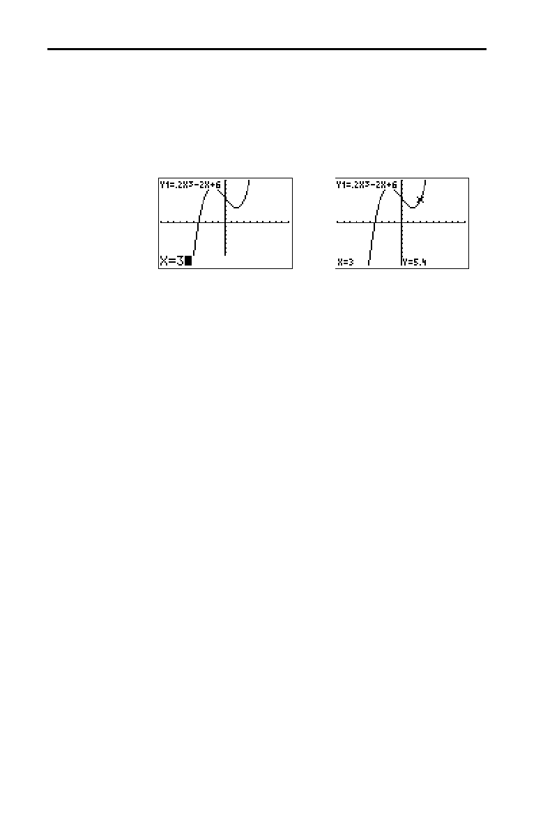
Function Graphing 3-19
8303FUNC.DOC TI-83 international English Bob Fedorisko Revised: 02/19/01 12:16 PM Printed: 02/19/01 1:35
PM Page 19 of 28
To move the trace cursor to any valid X value on the
current function, enter the value. When you enter the first
digit, an
X= prompt and the number you entered are
displayed in the bottom-left corner of the screen. You can
enter an expression at the
X= prompt. The value must be
valid for the current viewing window. When you have
completed the entry, press
Í
to move the cursor.
Note:
This feature does not apply to stat plots.
If you trace a function beyond the left or right side of the
screen, the viewing window automatically pans to the left
or right.
Xmin and Xmax are updated to correspond to the
new viewing window.
While tracing, you can press
Í
to adjust the viewing
window so that the cursor location becomes the center of
the new viewing window, even if the cursor is above or
below the display. This allows panning up and down. After
Quick Zoom, the cursor remains in
TRACE
.
When you leave and return to
TRACE
, the trace cursor is
displayed in the same location it was in when you left
TRACE
, unless Smart Graph has replotted the graph
(page 3
.
15).
On a blank line in the program editor, press
r
. The
instruction
Trace is pasted to the cursor location. When the
instruction is encountered during program execution, the
graph is displayed with the trace cursor on the first
selected function. As you trace, the cursor coordinate
values are updated. When you finish tracing the functions,
press
Í
to resume program execution.
Moving the Trace
Cursor to Any
Valid X Value
Panning to the
Left or Right
Quick Zoom
Leaving and
Returning to
TRACE
Using TRACE in
a Program
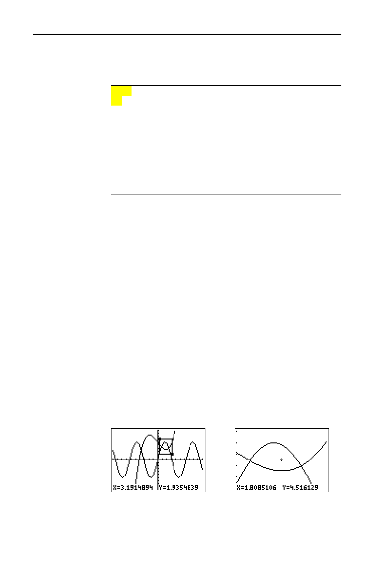
3-20 Function Graphing
8303FUNC.DOC TI-83 international English Bob Fedorisko Revised: 02/19/01 12:16 PM Printed: 02/19/01 1:35
PM Page 20 of 28
8303FUNC.DOC TI-83 international English Bob Fedorisko Revised: 02/19/01 12:16 PM Printed: 02/19/01 1:35
PM Page 20 of 28
To display the
ZOOM
menu, press
q
. You can adjust the
viewing window of the graph quickly in several ways. All
ZOOM
instructions are accessible from programs.
ZOOM MEMORY
1: ZBox
Draws a box to define the viewing window.
2: Zoom In
Magnifies the graph around the cursor.
3: Zoom Out
Views more of a graph around the cursor.
4: ZDecimal
Sets
@
X and
@
Y to 0.1.
5: ZSquare
Sets equal-size pixels on the X and Y axes.
6: ZStandard
Sets the standard window variables.
7: ZTrig
Sets the built-in trig window variables.
8: ZInteger
Sets integer values on the X and Y axes.
9: ZoomStat
Sets the values for current stat lists.
0: ZoomFit
Fits YMin and YMax between XMin and XMax.
When you select
1:ZBox, 2:Zoom In, or 3:Zoom Out, the
cursor on the graph becomes the zoom cursor (
+
), a
smaller version of the free-moving cursor (
+).
To define a new viewing window using
ZBox, follow these
steps.
1. Select
1:ZBox from the
ZOOM
menu. The zoom cursor is
displayed at the center of the screen.
2. Move the zoom cursor to any spot you want to define as
a corner of the box, and then press
Í
. When you
move the cursor away from the first defined corner, a
small, square dot indicates the spot.
3. Press
|
,
}
,
~
, or
†
. As you move the cursor, the sides
of the box lengthen or shorten proportionately on the
screen.
Note:
To cancel
ZBox
before you press
Í
, press
‘
.
4. When you have defined the box, press
Í
to replot
the graph.
To use ZBox to define another box within the new graph,
repeat steps 2 through 4. To cancel
ZBox, press
‘
.
Exploring Graphs with the ZOOM Instructions
ZOOM Menu
Zoom Cursor
ZBox

Function Graphing 3-21
8303FUNC.DOC TI-83 international English Bob Fedorisko Revised: 02/19/01 12:16 PM Printed: 02/19/01 1:35
PM Page 21 of 28
Zoom In magnifies the part of the graph that surrounds the
cursor location.
Zoom Out displays a greater portion of the
graph, centered on the cursor location. The
XFact and
YFact settings determine the extent of the zoom.
To zoom in on a graph, follow these steps.
1. Check
XFact and YFact (page 3
.
24); change as needed.
2. Select
2:Zoom In from the
ZOOM
menu. The zoom
cursor is displayed.
3. Move the zoom cursor to the point that is to be the
center of the new viewing window.
4. Press
Í
. The TI
-
83 adjusts the viewing window by
XFact and YFact; updates the window variables; and
replots the selected functions, centered on the cursor
location.
5. Zoom in on the graph again in either of two ways.
•
To zoom in at the same point, press
Í
.
•
To zoom in at a new point, move the cursor to the
point that you want as the center of the new viewing
window, and then press
Í
.
To zoom out on a graph, select
3:Zoom Out and repeat
steps 3 through 5.
To cancel
Zoom In or Zoom Out, press
‘
.
ZDecimal replots the functions immediately. It updates the
window variables to preset values, as shown below. These
values set
@
X and
@
Y equal to 0.1 and set the X and Y value
of each pixel to one decimal place.
Xmin=
L
4.7 Ymin=
L
3.1
Xmax=4.7 Ymax=3.1
Xscl=1 Yscl=1
ZSquare
replots the functions immediately. It redefines the
viewing window based on the current values of the
window variables. It adjusts in only one direction so that
@
X=
@
Y
, which makes the graph of a circle look like a circle.
Xscl and Yscl remain unchanged. The midpoint of the
current graph (not the intersection of the axes) becomes
the midpoint of the new graph.
Zoom In,
Zoom Out
ZDecimal
ZSquare

3-22 Function Graphing
8303FUNC.DOC TI-83 international English Bob Fedorisko Revised: 02/19/01 12:16 PM Printed: 02/19/01 1:35
PM Page 22 of 28
8303FUNC.DOC TI-83 international English Bob Fedorisko Revised: 02/19/01 12:16 PM Printed: 02/19/01 1:35
PM Page 22 of 28
ZStandard replots the functions immediately. It updates the
window variables to the standard values shown below.
Xmin=
L
10 Ymin=
L
10 Xres=1
Xmax=10 Ymax=10
Xscl=1 Yscl=1
ZTrig
replots the functions immediately. It updates the
window variables to preset values that are appropriate for
plotting trig functions. Those preset values in
Radian mode
are shown below.
Xmin=
L
(47
à
24)
p
Ymin=
L
4
Xmax=(47
à
24)
p
Ymax=4
Xscl=
p
/2 Yscl=1
ZInteger
redefines the viewing window to the dimensions
shown below. To use
ZInteger, move the cursor to the point
that you want to be the center of the new window, and
then press
Í
;
ZInteger replots the functions.
@
X=1 Xscl=10
@
Y=1 Yscl=10
ZoomStat
redefines the viewing window so that all
statistical data points are displayed. For regular and
modified box plots, only
Xmin and Xmax are adjusted.
ZoomFit replots the functions immediately. ZoomFit
recalculates YMin and YMax to include the minimum and
maximum
Y values of the selected functions between the
current
XMin and XMax. XMin and XMax are not changed.
ZStandard
ZTrig
ZInteger
ZoomStat
ZoomFit

Function Graphing 3-23
8303FUNC.DOC TI-83 international English Bob Fedorisko Revised: 02/19/01 12:16 PM Printed: 02/19/01 1:35
PM Page 23 of 28
To display the
ZOOM MEMORY
menu, press
q
~
.
ZOOM MEMORY
1:ZPrevious
Uses the previous viewing window.
2:ZoomSto
Stores the user-defined window.
3:ZoomRcl
Recalls the user-defined window.
4:SetFactors
...
Changes
Zoom In
and
Zoom Out
factors.
ZPrevious
replots the graph using the window variables of
the graph that was displayed before you executed the last
ZOOM
instruction.
ZoomSto
immediately stores the current viewing window.
The graph is displayed, and the values of the current
window variables are stored in the user-defined
ZOOM
variables
ZXmin
,
ZXmax
,
ZXscl
,
ZYmin
,
ZYmax
,
ZYscl
, and
ZXres
.
These variables apply to all graphing modes. For example,
changing the value of
ZXmin
in
Func
mode also changes it
in
Par
mode.
ZoomRcl
graphs the selected functions in a user-defined
viewing window. The user-defined viewing window is
determined by the values stored with the
ZoomSto
instruction. The window variables are updated with the
user-defined values, and the graph is plotted.
Using ZOOM MEMORY
ZOOM MEMORY
Menu
ZPrevious
ZoomSto
ZoomRcl
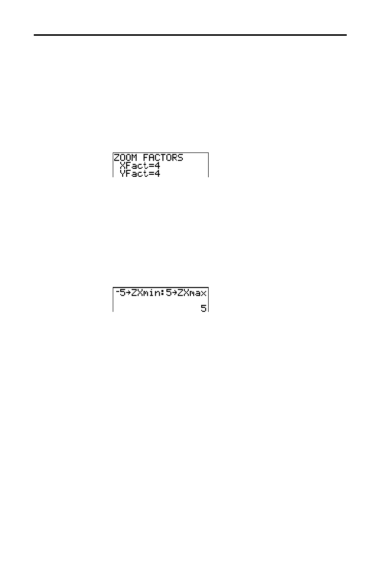
3-24 Function Graphing
8303FUNC.DOC TI-83 international English Bob Fedorisko Revised: 02/19/01 12:16 PM Printed: 02/19/01 1:35
PM Page 24 of 28
8303FUNC.DOC TI-83 international English Bob Fedorisko Revised: 02/19/01 12:16 PM Printed: 02/19/01 1:35
PM Page 24 of 28
The zoom factors, XFact and YFact, are positive numbers
(not necessarily integers) greater than or equal to 1. They
define the magnification or reduction factor used to
Zoom
In
or Zoom Out around a point.
To display the
ZOOM FACTORS
screen, where you can
review the current values for
XFact and YFact, select
4:SetFactors from the
ZOOM MEMORY
menu. The values
shown are the defaults.
You can change XFact and YFact in either of two ways.
•
Enter a new value. The original value is cleared
automatically when you enter the first digit.
•
Place the cursor on the digit you want to change, and
then enter a value or press
{
to delete it.
From the home screen or a program, you can store directly
to any of the user-defined
ZOOM
variables.
From a program, you can select the ZoomSto and ZoomRcl
instructions from the
ZOOM MEMORY
menu.
ZOOM FACTORS
Checking XFact
and YFact
Changing XFact
and YFact
Using ZOOM
MEMORY Menu
Items from the
Home Screen or
a Program
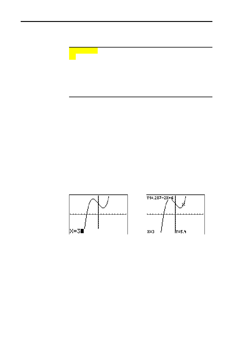
Function Graphing 3-25
8303FUNC.DOC TI-83 international English Bob Fedorisko Revised: 02/19/01 12:16 PM Printed: 02/19/01 1:35
PM Page 25 of 28
To display the
CALCULATE
menu, press
y
ã
CALCä
. Use the
items on this menu to analyze the current graph functions.
CALCULATE
1: value
Calculates a function Y value for a given X.
2: zero
Finds a zero (x-intercept) of a function.
3: minimum
Finds a minimum of a function.
4: maximum
Finds a maximum of a function.
5: intersect
Finds an intersection of two functions.
6: dy/dx
Finds a numeric derivative of a function.
7:
‰
f(x)dx
Finds a numeric integral of a function.
value evaluates one or more currently selected functions
for a specified value of
X.
Note:
When a value is displayed for
X
, press
‘
to clear the value.
When no value is displayed, press
‘
to cancel the
value
operation.
To evaluate a selected function at X, follow these steps.
1. Select
1:value from the
CALCULATE
menu. The graph is
displayed with
X= in the bottom-left corner.
2. Enter a real value, which can be an expression, for
X
between Xmin and Xmax.
3. Press
Í
.
The cursor is on the first selected function in the
Y=
editor
at the
X value you entered, and the coordinates are
displayed, even if
CoordOff format is selected.
To move the cursor from function to function at the
entered
X value, press
}
or
†
. To restore the free-moving
cursor, press
|
or
~
.
Using the CALC (Calculate) Operations
CALCULATE
Menu
value
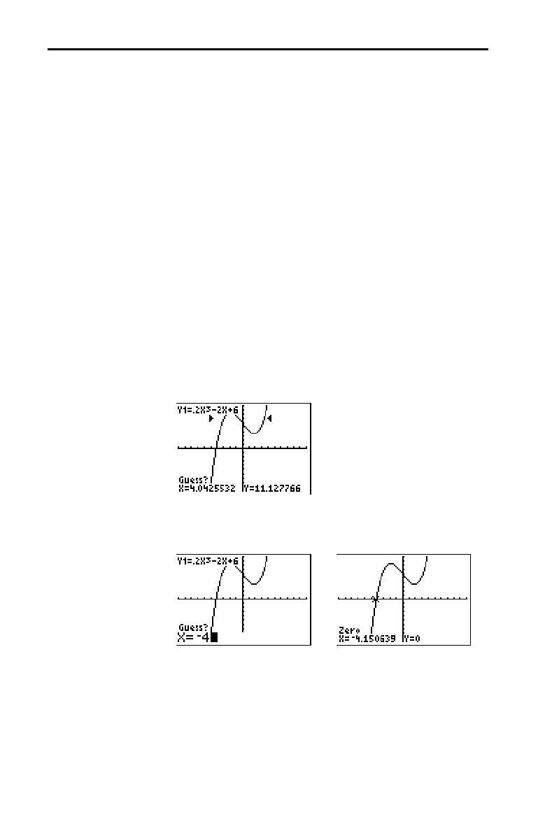
3-26 Function Graphing
8303FUNC.DOC TI-83 international English Bob Fedorisko Revised: 02/19/01 12:16 PM Printed: 02/19/01 1:35
PM Page 26 of 28
8303FUNC.DOC TI-83 international English Bob Fedorisko Revised: 02/19/01 12:16 PM Printed: 02/19/01 1:35
PM Page 26 of 28
zero finds a zero (x-intercept or root) of a function using
solve(. Functions can have more than one x-intercept
value;
zero finds the zero closest to your guess.
The time
zero spends to find the correct zero value
depends on the accuracy of the values you specify for the
left and right bounds and the accuracy of your guess.
To find a zero of a function, follow these steps.
1. Select
2:zero from the
CALCULATE
menu. The current
graph is displayed with
Left Bound?
in the bottom-left
corner.
2. Press
}
or
†
to move the cursor onto the function for
which you want to find a zero.
3. Press
|
or
~
(or enter a value) to select the x-value for
the left bound of the interval, and then press
Í
. A
4
indicator on the graph screen shows the left bound.
Right Bound? is displayed in the bottom-left corner.
Press
|
or
~
(or enter a value) to select the x-value for
the right bound, and then press
Í
. A
3
indicator on
the graph screen shows the right bound.
Guess? is then
displayed in the bottom-left corner.
4. Press
|
or
~
(or enter a value) to select a point near
the zero of the function, between the bounds, and then
press
Í
.
The cursor is on the solution and the coordinates are
displayed, even if
CoordOff format is selected. To move to
the same x-value for other selected functions, press
}
or
†
. To restore the free-moving cursor, press
|
or
~
.
zero
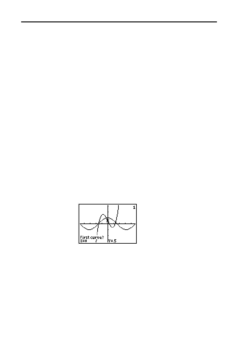
Function Graphing 3-27
8303FUNC.DOC TI-83 international English Bob Fedorisko Revised: 02/19/01 12:16 PM Printed: 02/19/01 1:35
PM Page 27 of 28
minimum and maximum find a minimum or maximum of a
function within a specified interval to a tolerance of 1
âL
5.
To find a minimum or maximum, follow these steps.
1. Select
3:minimum or 4:maximum from the
CALCULATE
menu. The current graph is displayed.
2. Select the function and set left bound, right bound, and
guess as described for
zero (steps 2 through 4; page 3
.
26).
The cursor is on the solution, and the coordinates are
displayed, even if you have selected
CoordOff format;
Minimum or Maximum is displayed in the bottom-left
corner.
To move to the same x-value for other selected functions,
press
}
or
†
. To restore the free-moving cursor, press
|
or
~
.
intersect finds the coordinates of a point at which two or
more functions intersect using
solve(. The intersection
must appear on the display to use
intersect.
To find an intersection, follow these steps.
1. Select
5:intersect from the
CALCULATE
menu. The
current graph is displayed with
First curve?
in the
bottom-left corner.
2. Press
†
or
}
, if necessary, to move the cursor to the
first function, and then press
Í
.
Second curve? is
displayed in the bottom-left corner.
3. Press
†
or
}
, if necessary, to move the cursor to the
second function, and then press
Í
.
4. Press
~
or
|
to move the cursor to the point that is
your guess as to location of the intersection, and then
press
Í
.
The cursor is on the solution and the coordinates are
displayed, even if
CoordOff format is selected. Intersection
is displayed in the bottom-left corner. To restore the free-
moving cursor, press
|
,
}
,
~
, or
†
.
minimum,
maximum
intersect
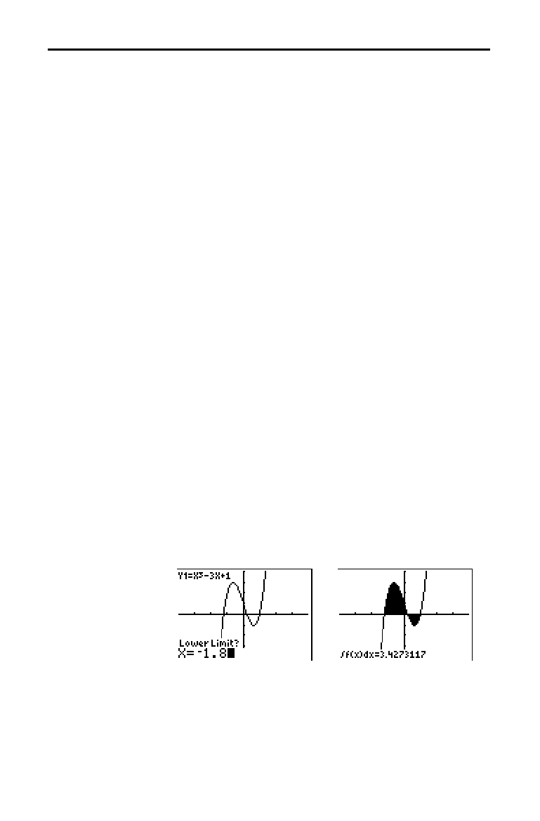
3-28 Function Graphing
8303FUNC.DOC TI-83 international English Bob Fedorisko Revised: 02/19/01 12:16 PM Printed: 02/19/01 1:35
PM Page 28 of 28
8303FUNC.DOC TI-83 international English Bob Fedorisko Revised: 02/19/01 12:16 PM Printed: 02/19/01 1:35
PM Page 28 of 28
dy/dx (numerical derivative) finds the numerical derivative
(slope) of a function at a point, with
H
=1
âL
3.
To find a function’s slope at a point, follow these steps.
1. Select
6:dy/dx from the
CALCULATE
menu. The current
graph is displayed.
2. Press
}
or
†
to select the function for which you want
to find the numerical derivative.
3. Press
|
or
~
(or enter a value) to select the
X value at
which to calculate the derivative, and then press
Í
.
The cursor is on the solution and the numerical derivative
is displayed.
To move to the same x-value for other selected functions,
press
}
or
†
. To restore the free-moving cursor, press
|
or
~
.
‰
f(x)dx
(numerical integral) finds the numerical integral of a
function in a specified interval. It uses the
fnInt( function,
with a tolerance of
H
=1
âL
3.
To find the numerical derivative of a function, follow these
steps.
1. Select
7:
‰
f(x)dx from the
CALCULATE
menu. The current
graph is displayed with
Lower Limit? in the bottom-left
corner.
2. Press
}
or
†
to move the cursor to the function for
which you want to calculate the integral.
3. Set lower and upper limits as you would set left and
right bounds for
zero (step 3; page 3
.
26). The integral
value is displayed, and the integrated area is shaded.
Note:
The shaded area is a drawing. Use
ClrDraw
(Chapter 8) or
any action that invokes Smart Graph to clear the shaded area.
dy/dx
‰
f(x)dx
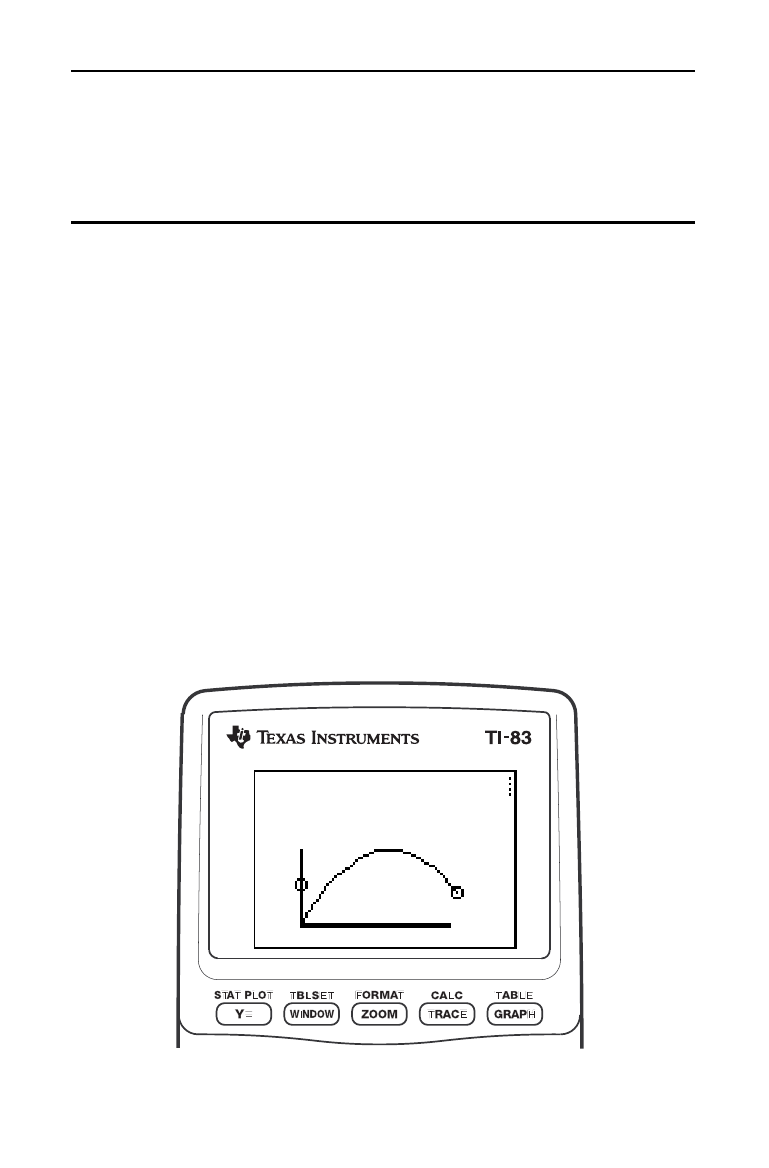
Parametric Graphing 4-1
8304PARA.DOC TI-83 international English Bob Fedorisko Revised: 02/19/01 12:17 PM Printed: 02/19/01 1:36
PM Page 1 of 8
4
Parametric
Graphin
g
Getting Started: Path of a Ball
...........................
4-2
Defining and Displaying Parametric Graphs
..............
4-4
Exploring Parametric Graphs
............................
4-7
Contents
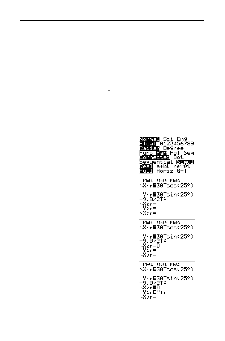
4-2 Parametric Graphing
8304PARA.DOC TI-83 international English Bob Fedorisko Revised: 02/19/01 12:17 PM Printed: 02/19/01 1:36
PM Page 2 of 8
Getting Started is a fast-paced introduction. Read the chapter for details.
Graph the parametric equation that describes the path of a ball hit at an initial
speed of 30 meters per second, at an initial angle of 25 degrees with the
horizontal from ground level. How far does the ball travel? When does it hit the
ground? How high does it go? Ignore all forces except gravity.
For initial velocity v
0
and angle
q
, the position of the ball as a function of time
has horizontal and vertical components.
Horizontal: X1(t)=tv
0
cos(
q
)
Vertical: Y1(t)=tv
0
sin(
q
)
N
1
2
gt
2
The vertical and horizontal vectors of the ball’s motion also will be graphed.
Vertical vector: X2(t)=0 Y2(t)=Y1(t)
Horizontal vector: X3(t)=X1(t) Y3(t)=0
Gravity constant: g=9.8 m/sec
2
1. Press
z
. Press
†
†
†
~
Í
to
select
Par mode. Press
†
†
~
Í
to
select
Simul for simultaneous graphing of
all three parametric equations in this
example.
2. Press
o
. Press 30
„
™
25
y
[
ANGLE
] 1 (to select
¡
)
¤
Í
to define
X
1T
in terms of T.
3. Press
30
„
˜
25
y
[
ANGLE
] 1
¤
¹
9.8
¥
2
„
¡
Í
to define Y
1T
.
The vertical component vector is defined
by
X
2T
and Y
2T
.
4. Press
0
Í
to define X
2T
.
5. Press
~
to display the
VARS Y
.
VARS
menu. Press 2 to display the
PARAMETRIC
secondary menu. Press 2
Í
to define
Y
2T
.
Getting Started: Path of a Ball
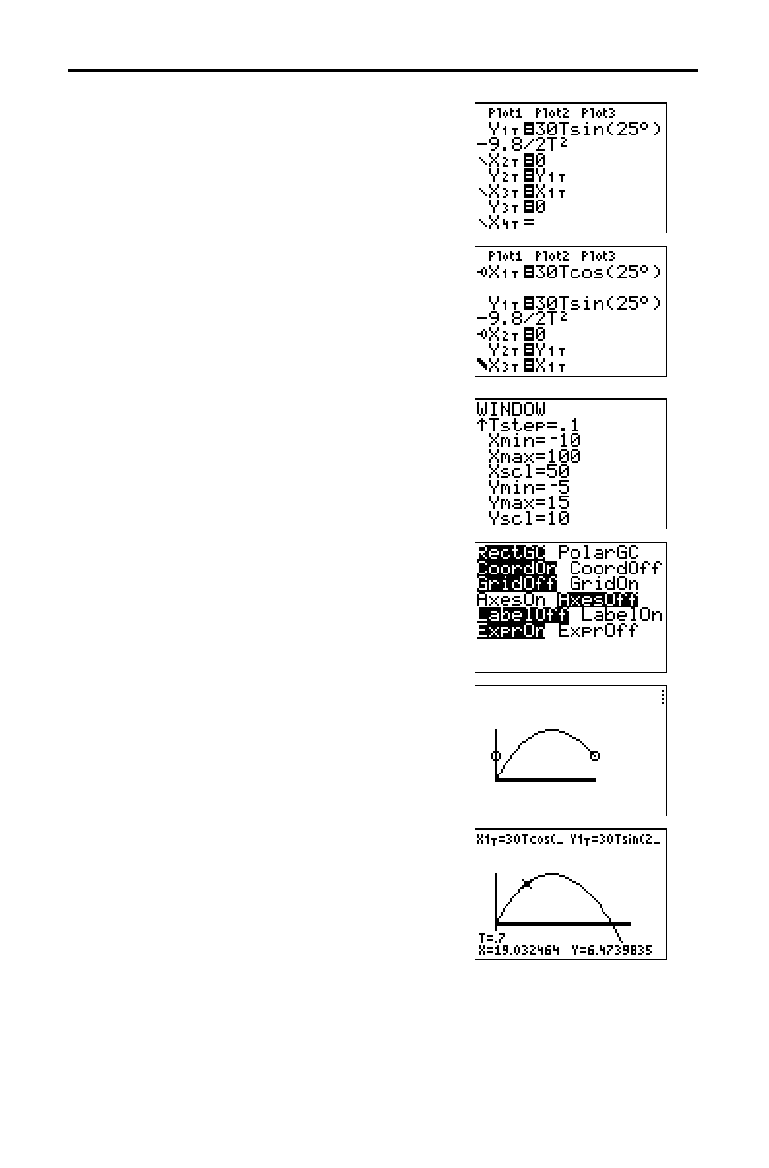
Parametric Graphing 4-3
8304PARA.DOC TI-83 international English Bob Fedorisko Revised: 02/19/01 12:17 PM Printed: 02/19/01 1:36
PM Page 3 of 8
The horizontal component vector is
defined by
X
3T
and Y
3T
.
6. Press
~
2, and then press 1
Í
to
define
X
3T
. Press 0
Í
to define Y
3T
.
7. Press
|
|
}
Í
to change the graph
style to
è
for
X
3T
and Y
3T
. Press
}
Í
Í
to change the graph style to
ë
for
X
2T
and Y
2T
. Press
}
Í
Í
to
change the graph style to
ë
for
X
1T
and Y
1T
.
(These keystrokes assume that all graph
styles were set to
ç
originally.)
8. Press
p
. Enter these values for the
window variables.
Tmin=0 Xmin=
L
10 Ymin=
L
5
Tmax=5 Xmax=100 Ymax=15
Tstep=.1 Xscl=50 Yscl=10
9. Press
y
[
FORMAT
]
†
†
†
~
Í
to set
AxesOff, which turns off the axes.
10. Press
s
. The plotting action
simultaneously shows the ball in flight and
the vertical and horizontal component
vectors of the motion.
Tip:
To simulate the ball flying through the air, set
graph style to
ì
(animate) for
X
1T
and
Y
1T
.
11. Press
r
to obtain numerical results
and answer the questions at the beginning
of this section.
Tracing begins at
Tmin on the first
parametric equation (
X
1T
and Y
1T
). As you
press
~
to trace the curve, the cursor
follows the path of the ball over time. The
values for
X (distance), Y (height), and T
(time) are displayed at the bottom of the
screen.
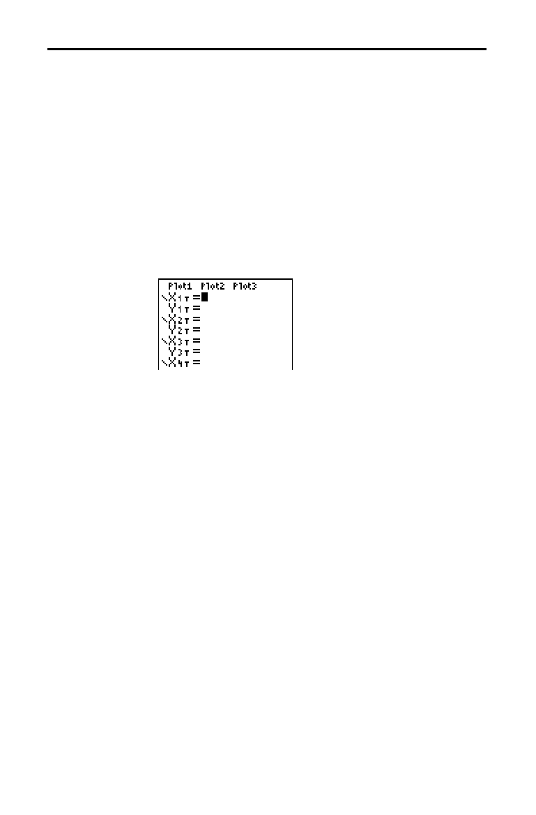
4-4 Parametric Graphing
8304PARA.DOC TI-83 international English Bob Fedorisko Revised: 02/19/01 12:17 PM Printed: 02/19/01 1:36
PM Page 4 of 8
The steps for defining a parametric graph are similar to the
steps for defining a function graph. Chapter 4 assumes that
you are familiar with Chapter 3: Function Graphing.
Chapter 4 details aspects of parametric graphing that differ
from function graphing.
To display the mode screen, press
z
. To graph
parametric equations, you must select
Par graphing mode
before you enter window variables and before you enter
the components of parametric equations.
After selecting
Par graphing mode, press
o
to display the
parametric
Y=
editor.
In this editor, you can display and enter both the X and Y
components of up to six equations, X
1T
and Y
1T
through X
6T
and Y
6T
. Each is defined in terms of the independent
variable
T. A common application of parametric graphs is
graphing equations over time.
The icons to the left of
X
1T
through X
6T
represent the graph
style of each parametric equation (Chapter 3). The default
in
Par mode is
ç
(line), which connects plotted points. Line,
è
(thick),
ë
(path),
ì
(animate), and
í
(dot) styles are
available for parametric graphing.
Defining and Displaying Parametric Graphs
TI-83 Graphing
Mode Similarities
Setting
Parametric
Graphing Mode
Displaying the
Parametric Y=
Editor
Selecting a
Graph Style

Parametric Graphing 4-5
8304PARA.DOC TI-83 international English Bob Fedorisko Revised: 02/19/01 12:17 PM Printed: 02/19/01 1:36
PM Page 5 of 8
To define or edit a parametric equation, follow the steps in
Chapter 3 for defining a function or editing a function. The
independent variable in a parametric equation is
T. In Par
graphing mode, you can enter the parametric variable T in
either of two ways.
•
Press
„
.
•
Press
ƒ
ã
Tä
.
Two components,
X and Y, define a single parametric
equation. You must define both of them.
The TI
-
83 graphs only the selected parametric equations.
In the
Y=
editor, a parametric equation is selected when the
= signs of both the X and Y components are highlighted.
You may select any or all of the equations
X
1T
and Y
1T
through X
6T
and Y
6T
.
To change the selection status, move the cursor onto the =
sign of either the
X or Y component and press
Í
. The
status of both the
X and Y components is changed.
To display the window variable values, press
p
.
These variables define the viewing window. The values
below are defaults for
Par graphing in Radian angle mode.
Tmin=0
Smallest T value to evaluate
Tmax=6.2831853
...
Largest T value to evaluate (2
p
)
Tstep=.1308996
...
T value increment (
pà
24)
Xmin=
L
10
Smallest X value to be displayed
Xmax=10
Largest X value to be displayed
Xscl=1
Spacing between the X tick marks
Ymin=
L
10
Smallest Y value to be displayed
Ymax=10
Largest Y value to be displayed
Yscl=1
Spacing between the Y tick marks
Note:
To ensure that sufficient points are plotted, you may want to
change the
T
window variables.
Defining and
Editing
Parametric
Equations
Selecting and
Deselecting
Parametric
Equations
Setting Window
Variables
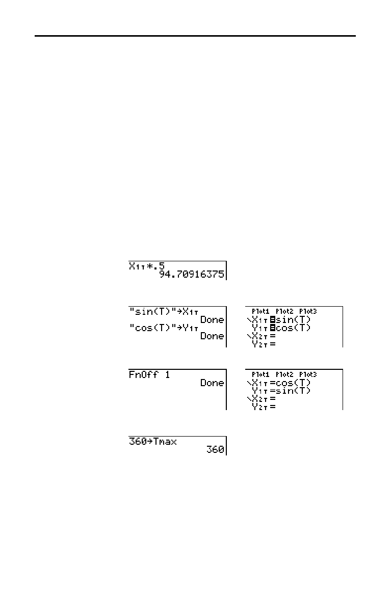
4-6 Parametric Graphing
8304PARA.DOC TI-83 international English Bob Fedorisko Revised: 02/19/01 12:17 PM Printed: 02/19/01 1:36
PM Page 6 of 8
To display the current graph format settings, press
y
[
FORMAT
]. Chapter 3 describes the format settings in detail.
The other graphing modes share these format settings;
Seq
graphing mode has an additional axes format setting.
When you press
s
, the TI
-
83 plots the selected
parametric equations. It evaluates the
X and Y components
for each value of
T (from Tmin to Tmax in intervals of
Tstep), and then plots each point defined by X and Y. The
window variables define the viewing window.
As the graph is plotted,
X, Y, and T are updated.
Smart Graph applies to parametric graphs (Chapter 3).
You can perform these actions from the home screen or a
program.
•
Access functions by using the name of the
X or Y
component of the equation as a variable.
•
Store parametric equations.
•
Select or deselect parametric equations.
•
Store values directly to window variables.
Setting the Graph
Format
Displaying a
Graph
Window
Variables and
Y-VARS Menus

Parametric Graphing 4-7
8304PARA.DOC TI-83 international English Bob Fedorisko Revised: 02/19/01 12:17 PM Printed: 02/19/01 1:36
PM Page 7 of 8
The free-moving cursor in Par graphing works the same as
in
Func graphing.
In
RectGC format, moving the cursor updates the values of
X and Y; if CoordOn format is selected, X and Y are
displayed.
In
PolarGC format, X, Y, R, and
q
are updated; if CoordOn
format is selected, R and
q
are displayed.
To activate
TRACE
, press
r
. When
TRACE
is active,
you can move the trace cursor along the graph of the
equation one
Tstep at a time. When you begin a trace, the
trace cursor is on the first selected function at
Tmin. If
ExprOn is selected, then the function is displayed.
In
RectGC format,
TRACE
updates and displays the values
of
X, Y, and T if CoordOn format is on.
In
PolarGC format, X, Y, R,
q
and T are updated; if CoordOn
format is selected, R,
q
, and T are displayed. The X and Y
(or R and
q
) values are calculated from T.
To move five plotted points at a time on a function, press
y
|
or
y
~
. If you move the cursor beyond the top or
bottom of the screen, the coordinate values at the bottom
of the screen continue to change appropriately.
Quick Zoom is available in
Par graphing; panning is not
(Chapter 3).
Exploring Parametric Graphs
Free-Moving
Cursor
TRACE
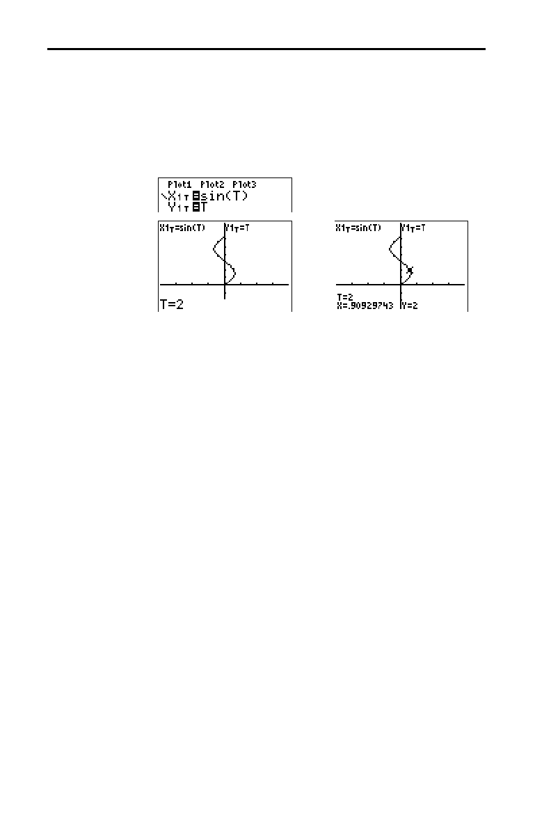
4-8 Parametric Graphing
8304PARA.DOC TI-83 international English Bob Fedorisko Revised: 02/19/01 12:17 PM Printed: 02/19/01 1:36
PM Page 8 of 8
To move the trace cursor to any valid T value on the
current function, enter the number. When you enter the
first digit, a
T= prompt and the number you entered are
displayed in the bottom-left corner of the screen. You can
enter an expression at the
T= prompt. The value must be
valid for the current viewing window. When you have
completed the entry, press
Í
to move the cursor.
ZOOM
operations in Par graphing work the same as in Func
graphing. Only the X (Xmin, Xmax, and Xscl) and Y (Ymin,
Ymax, and Yscl) window variables are affected.
The
T window variables (Tmin, Tmax, and Tstep) are only
affected when you select
ZStandard. The
VARS ZOOM
secondary menu
ZT/Z
q
items 1:ZTmin, 2:ZTmax, and
3:ZTstep are the zoom memory variables for Par graphing.
CALC
operations in Par graphing work the same as in Func
graphing. The
CALCULATE
menu items available in Par
graphing are 1:value, 2:dy/dx, 3:dy/dt, and 4:dx/dt.
Moving the Trace
Cursor to Any
Valid T Value
ZOOM
CALC
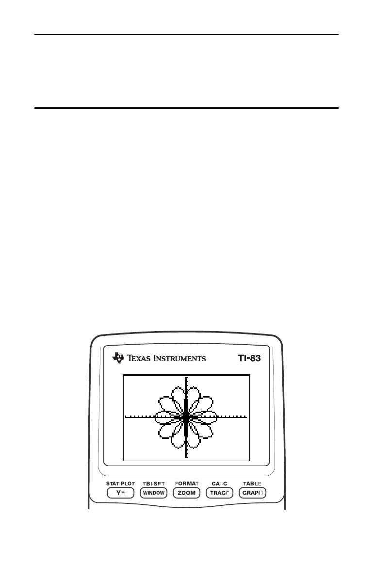
Polar Graphing 5-1
8305POLR.DOC TI-83 international English Bob Fedorisko Revised: 02/19/01 12:19 PM Printed: 02/19/01 1:36
PM Page 1 of 6
5
Polar
Graphin
g
Getting Started: Polar Rose
..............................
5-2
Defining and Displaying Polar Graphs
...................
5-3
Exploring Polar Graphs
..................................
5-6
Contents
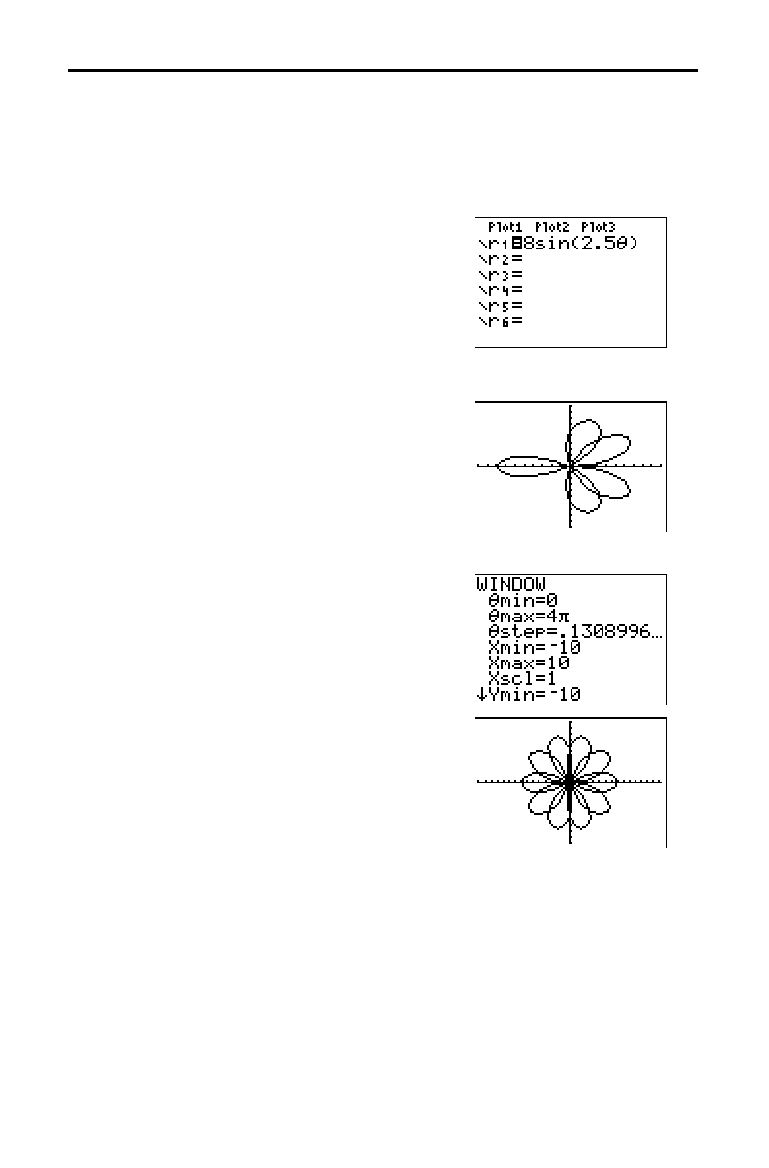
5-2 Polar Graphing
8305POLR.DOC TI-83 international English Bob Fedorisko Revised: 02/19/01 12:19 PM Printed: 02/19/01 1:36
PM Page 2 of 6
Getting Started is a fast-paced introduction. Read the chapter for details.
The polar equation R=Asin(B
q
) graphs a rose. Graph the rose for A=8 and
B=2.5, and then explore the appearance of the rose for other values of A and B.
1. Press
z
to display the mode screen.
Press
†
†
†
~
~
Í
to select
Pol
graphing mode. Select the defaults (the
options on the left) for the other mode
settings.
2. Press
o
to display the polar
Y=
editor.
Press
8
˜
2.5
„
¤
Í
to define
r
1
.
3. Press
q
6 to select 6:ZStandard and
graph the equation in the standard viewing
window. The graph shows only five petals
of the rose, and the rose does not appear
to be symmetrical. This is because the
standard window sets
q
max=2
p
and defines
the window, rather than the pixels, as
square.
4. Press
p
to display the window
variables. Press
†
4
y
[
p
] to increase the
value of
q
max
to 4
p
.
5. Press
q
5 to select 5:ZSquare and plot
the graph.
6. Repeat steps 2 through 5 with new values
for the variables
A and B in the polar
equation
r
1
=Asin(B
q
). Observe how the new
values affect the graph.
Getting Started: Polar Rose
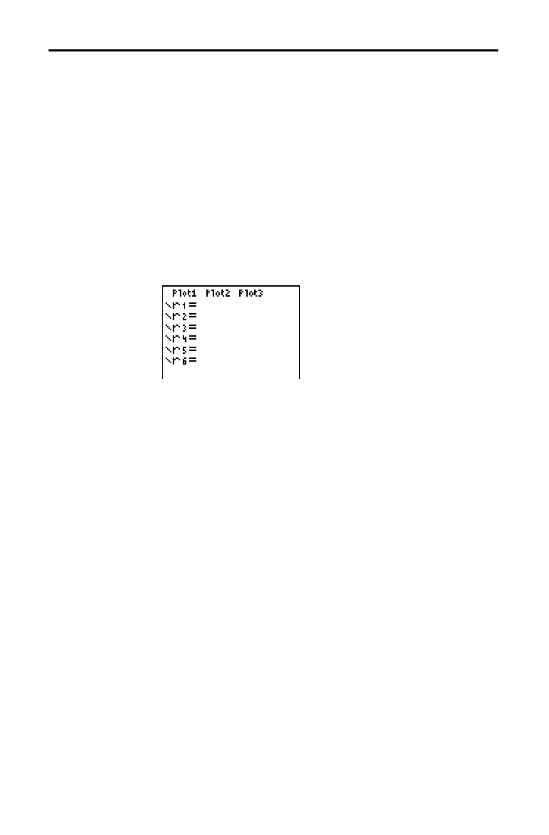
Polar Graphing 5-3
8305POLR.DOC TI-83 international English Bob Fedorisko Revised: 02/19/01 12:19 PM Printed: 02/19/01 1:36
PM Page 3 of 6
The steps for defining a polar graph are similar to the steps
for defining a function graph. Chapter 5 assumes that you
are familiar with Chapter 3: Function Graphing. Chapter 5
details aspects of polar graphing that differ from function
graphing.
To display the mode screen, press
z
. To graph polar
equations, you must select
Pol graphing mode before you
enter values for the window variables and before you enter
polar equations.
After selecting
Pol graphing mode, press
o
to display the
polar
Y=
editor.
In this editor, you can enter and display up to six polar
equations,
r
1
through r
6
. Each is defined in terms of the
independent variable
q
(page 5
.
4).
The icons to the left of
r
1
through r
6
represent the graph
style of each polar equation (Chapter 3). The default in
Pol
graphing mode is
ç
(line), which connects plotted points.
Line,
è
(thick),
ë
(path),
ì
(animate), and
í
(dot) styles are
available for polar graphing.
Defining and Displaying Polar Graphs
TI-83 Graphing
Mode Similarities
Setting Polar
Graphing Mode
Displaying the
Polar Y= Editor
Selecting Graph
Styles

5-4 Polar Graphing
8305POLR.DOC TI-83 international English Bob Fedorisko Revised: 02/19/01 12:19 PM Printed: 02/19/01 1:36
PM Page 4 of 6
To define or edit a polar equation, follow the steps in
Chapter 3 for defining a function or editing a function. The
independent variable in a polar equation is
q
. In Pol
graphing mode, you can enter the polar variable
q
in either
of two ways.
•
Press
„
.
•
Press
ƒ
ãqä
.
The TI
-
83 graphs only the selected polar equations. In the
Y=
editor, a polar equation is selected when the = sign is
highlighted. You may select any or all of the equations.
To change the selection status, move the cursor onto the
= sign, and then press
Í
.
To display the window variable values, press
p
.
These variables define the viewing window. The values
below are defaults for
Pol graphing in Radian angle mode.
q
min=0
Smallest
q
value to evaluate
q
max=6.2831853
...
Largest
q
value to evaluate (2
p
)
q
step=.1308996
...
Increment between
q
values (
pà
24)
Xmin=
L
10
Smallest X value to be displayed
Xmax=10
Largest X value to be displayed
Xscl=1
Spacing between the X tick marks
Ymin=
L
10
Smallest Y value to be displayed
Ymax=10
Largest Y value to be displayed
Yscl=1
Spacing between the Y tick marks
Note:
To ensure that sufficient points are plotted, you may want to
change the
q
window variables.
Defining and
Editing Polar
Equations
Selecting and
Deselecting Polar
Equations
Setting Window
Variables
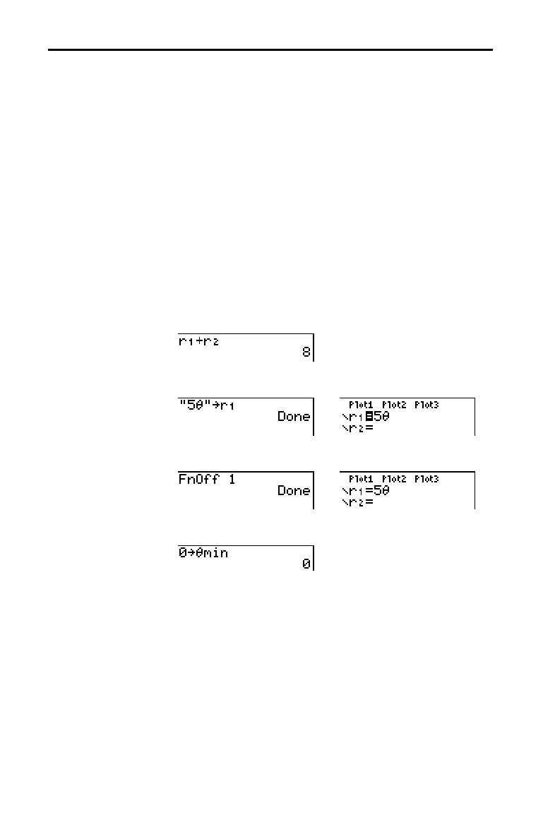
Polar Graphing 5-5
8305POLR.DOC TI-83 international English Bob Fedorisko Revised: 02/19/01 12:19 PM Printed: 02/19/01 1:36
PM Page 5 of 6
To display the current graph format settings, press
y
[
FORMAT
]. Chapter 3 describes the format settings in detail.
The other graphing modes share these format settings.
When you press
s
, the TI
-
83 plots the selected polar
equations. It evaluates
R for each value of
q
(from
q
min
to
q
max
in intervals of
q
step
) and then plots each point. The
window variables define the viewing window.
As the graph is plotted,
X, Y, R, and
q
are updated.
Smart Graph applies to polar graphs (Chapter 3).
You can perform these actions from the home screen or a
program.
•
Access functions by using the name of the equation as a
variable.
•
Store polar equations.
•
Select or deselect polar equations.
•
Store values directly to window variables.
Setting the Graph
Format
Displaying a
Graph
Window
Variables and
Y
.
VARS Menus

5-6 Polar Graphing
8305POLR.DOC TI-83 international English Bob Fedorisko Revised: 02/19/01 12:19 PM Printed: 02/19/01 1:36
PM Page 6 of 6
The free-moving cursor in Pol graphing works the same as
in
Func graphing. In RectGC format, moving the cursor
updates the values of
X and Y; if CoordOn format is
selected,
X and Y are displayed. In PolarGC format, X, Y, R,
and
q
are updated; if CoordOn format is selected, R and
q
are displayed.
To activate
TRACE
, press
r
. When
TRACE
is active,
you can move the trace cursor along the graph of the
equation one
q
step
at a time. When you begin a trace, the
trace cursor is on the first selected function at
q
min
. If
ExprOn format is selected, then the equation is displayed.
In
RectGC format,
TRACE
updates the values of X, Y, and
q
;
if
CoordOn format is selected, X, Y, and
q
are displayed. In
PolarGC format,
TRACE
updates X, Y, R, and
q
; if CoordOn
format is selected, R and
q
are displayed.
To move five plotted points at a time on a function, press
y
|
or
y
~
. If you move the trace cursor beyond the
top or bottom of the screen, the coordinate values at the
bottom of the screen continue to change appropriately.
Quick Zoom is available in
Pol graphing mode; panning is
not (Chapter 3).
To move the trace cursor to any valid
q
value on the
current function, enter the number. When you enter the
first digit, a
q
=
prompt and the number you entered are
displayed in the bottom-left corner of the screen. You can
enter an expression at the
q
=
prompt. The value must be
valid for the current viewing window. When you complete
the entry, press
Í
to move the cursor.
ZOOM
operations in Pol graphing work the same as in Func
graphing. Only the X (Xmin, Xmax, and Xscl) and Y (Ymin,
Ymax, and Yscl) window variables are affected.
The
q
window variables (
q
min
,
q
max
, and
q
step) are not
affected, except when you select
ZStandard. The
VARS
ZOOM
secondary menu
ZT/Z
q
items 4:Z
q
min, 5:Z
q
max, and
6:Z
q
step are zoom memory variables for Pol graphing.
CALC
operations in Pol graphing work the same as in Func
graphing. The
CALCULATE
menu items available in Pol
graphing are 1:value, 2:dy/dx, and 3:dr/d
q
.
Exploring Polar Graphs
Free-Moving
Cursor
TRACE
Moving the Trace
Cursor to Any
Valid
q
Value
ZOOM
CALC
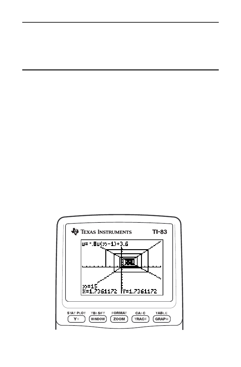
Sequence Graphing 6-1
8306SEQN.DOC TI-83 international English Bob Fedorisko Revised: 02/19/01 12:22 PM Printed: 02/19/01 1:36
PM Page 1 of 16
6
Sequence
Graphin
g
Getting Started: Forest and Trees
........................
6-2
Defining and Displaying Sequence Graphs
...............
6-3
Selecting Axes Combinations
............................
6-8
Exploring Sequence Graphs
..............................
6-9
Graphing Web Plots
......................................
6-11
Using Web Plots to Illustrate Convergence
...............
6-12
Graphing Phase Plots
....................................
6-13
Comparing TI
-
83 and TI
.
82 Sequence Variables
..........
6-15
Keystroke Differences Between TI
-
83 and TI
-
82
.........
6-16
Contents
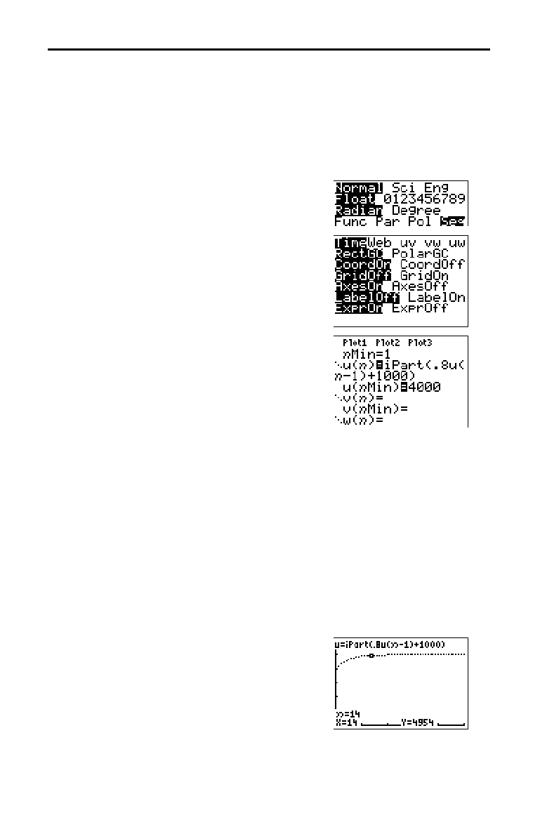
6-2 Sequence Graphing
8306SEQN.DOC TI-83 international English Bob Fedorisko Revised: 02/19/01 12:22 PM Printed: 02/19/01 1:36
PM Page 2 of 16
Getting Started is a fast-paced introduction. Read the chapter for details.
A small forest of 4,000 trees is under a new forestry plan. Each year 20 percent
of the trees will be harvested and 1,000 new trees will be planted. Will the
forest eventually disappear? Will the forest size stabilize? If so, in how many
years and with how many trees?
1. Press
z
. Press
†
†
†
~
~
~
Í
to select
Seq graphing mode.
2. Press
y
[
FORMAT
] and select Time axes
format and
ExprOn format if necessary.
3. Press
o
. If the graph-style icon is not
í
(dot), press
|
|
, press
Í
until
í
is
displayed, and then press
~
~
.
4. Press
~
3 to select iPart( (integer
part) because only whole trees are
harvested. After each annual harvest, 80
percent (.80) of the trees remain. Press
Ë
8
y
[
u
]
£
„
¹
1
¤
to define the
number of trees after each harvest. Press
Ã
1000
¤
to define the new trees. Press
†
4000 to define the number of trees at the
beginning of the program.
5. Press
p
0 to set
n
Min=0. Press
†
50
to set
n
Max=50.
n
Min and
n
Max evaluate
forest size over 50 years. Set the other
window variables.
PlotStart=1 Xmin=0 Ymin=0
PlotStep=1 Xmax=50 Ymax=6000
Xscl=10 Yscl=1000
6. Press
r
. Tracing begins at
n
Min (the
start of the forestry plan). Press
~
to trace
the sequence year by year. The sequence is
displayed at the top of the screen. The
values for
n
(number of years), X (X=
n
,
because
n
is plotted on the x-axis), and Y
(tree count) are displayed at the bottom.
When will the forest stabilize? With how
many trees?
Getting Started: Forest and Trees

Sequence Graphing 6-3
8306SEQN.DOC TI-83 international English Bob Fedorisko Revised: 02/19/01 12:22 PM Printed: 02/19/01 1:36
PM Page 3 of 16
The steps for defining a sequence graph are similar to the
steps for defining a function graph. Chapter 6 assumes that
you are familiar with Chapter 3: Function Graphing.
Chapter 6 details aspects of sequence graphing that differ
from function graphing.
To display the mode screen, press
z
. To graph
sequence functions, you must select
Seq graphing mode
before you enter window variables and before you enter
sequence functions.
Sequence graphs automatically plot in
Simul mode,
regardless of the current plotting-order mode setting.
The TI
-
83 has three sequence functions that you can enter
from the keyboard:
u, v, and w. They are above the
¬
,
−
,
and
®
keys.
You can define sequence functions in terms of:
•
The independent variable
n
•
The previous term in the sequence function, such as
u(
n
N
1)
•
The term that precedes the previous term in the
sequence function, such as
u(
n
N
2)
•
The previous term or the term that precedes the
previous term in another sequence function, such as
u(
n
N
1)
or u(
n
N
2)
referenced in the sequence v(
n
).
Note:
Statements in this chapter about
u(
n
)
are also true for
v(
n
)
and
w(
n
)
; statements about
u(
n
N
1)
are also true for
v(
n
N
1)
and
w(
n
N
1)
;
statements about
u(
n
N
2)
are also true for
v(
n
N
2)
and
w(
n
N
2)
.
Defining and Displaying Sequence Graphs
TI-83 Graphing
Mode Similarities
Setting Sequence
Graphing Mode
TI-83 Sequence
Functions u, v,
and w
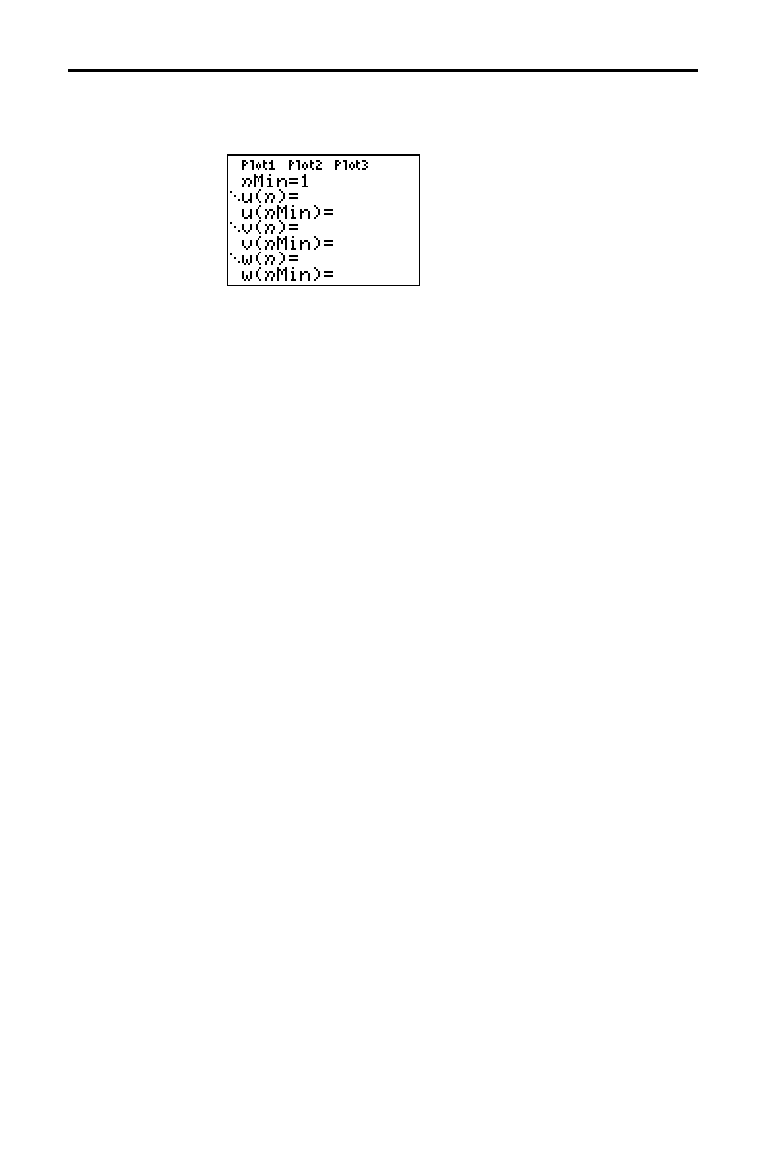
6-4 Sequence Graphing
8306SEQN.DOC TI-83 international English Bob Fedorisko Revised: 02/19/01 12:22 PM Printed: 02/19/01 1:36
PM Page 4 of 16
After selecting Seq mode, press
o
to display the sequence
Y=
editor.
In this editor, you can display and enter sequences for u(
n
),
v(
n
), and w(
n
). Also, you can edit the value for
n
Min, which
is the sequence window variable that defines the minimum
n
value to evaluate.
The sequence
Y=
editor displays the
n
Min value because of
its relevance to
u(
n
Min), v(
n
Min), and w(
n
Min), which are the
initial values for the sequence equations
u(
n
), v(
n
), and
w(
n
), respectively.
n
Min in the
Y=
editor is the same as
n
Min in the window
editor. If you enter a new value for
n
Min in one editor, the
new value for
n
Min is updated in both editors.
Note:
Use
u(
n
Min)
,
v(
n
Min)
, or
w(
n
Min)
only with a recursive
sequence, which requires an initial value.
The icons to the left of u(
n
), v(
n
), and w(
n
) represent the
graph style of each sequence (Chapter 3). The default in
Seq mode is
í
(dot), which shows discrete values. Dot,
ç
(line), and
è
(thick) styles are available for sequence
graphing. Graph styles are ignored in
Web format.
The TI
-
83 graphs only the selected sequence functions. In
the
Y=
editor, a sequence function is selected when the =
signs of both u(
n
)= and u(
n
Min)= are highlighted.
To change the selection status of a sequence function,
move the cursor onto the
= sign of the function name, and
then press
Í
. The status is changed for both the
sequence function
u(
n
) and its initial value u(
n
Min).
Displaying the
Sequence Y=
Editor
Selecting Graph
Styles
Selecting and
Deselecting
Sequence
Functions
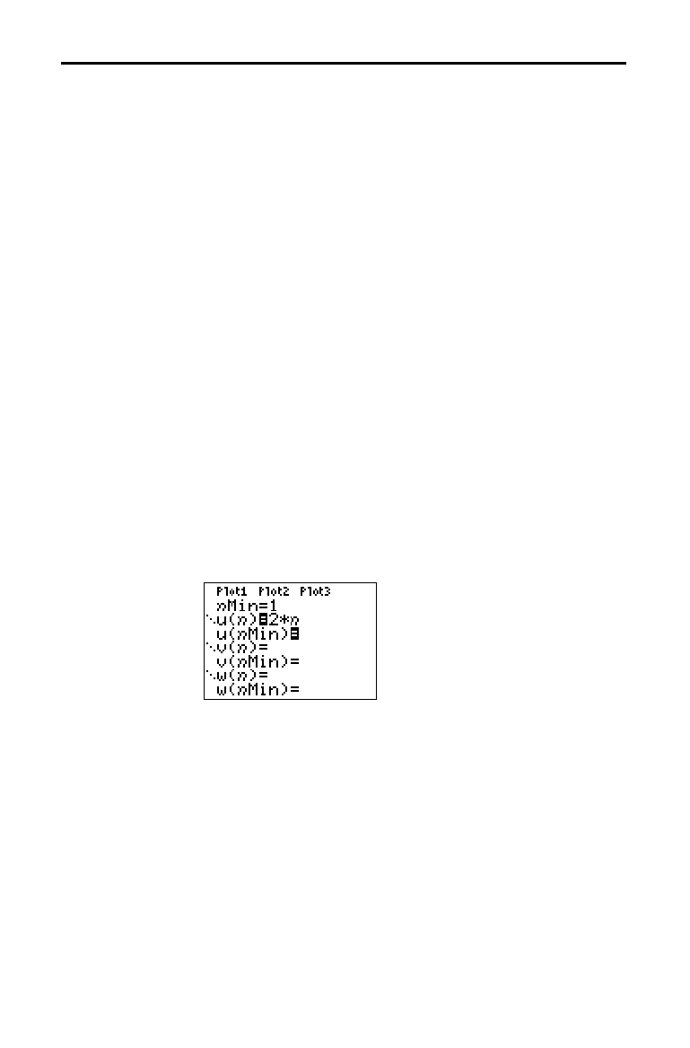
Sequence Graphing 6-5
8306SEQN.DOC TI-83 international English Bob Fedorisko Revised: 02/19/01 12:22 PM Printed: 02/19/01 1:36
PM Page 5 of 16
To define or edit a sequence function, follow the steps in
Chapter 3 for defining a function. The independent variable
in a sequence is
n
.
In
Seq graphing mode, you can enter the sequence variable
in either of two ways.
•
Press
„
.
•
Press
y
[
CATALOG
] [
N
].
You can enter the function name from the keyboard.
•
To enter the function name
u, press
y
[
u
] (above
¬
).
•
To enter the function name
v, press
y
[
v
] (above
−
).
•
To enter the function name
w, press
y
[
w
] (above
®
).
Generally, sequences are either nonrecursive or recursive.
Sequences are evaluated only at consecutive integer
values.
n
is always a series of consecutive integers, starting
at zero or any positive integer.
In a nonrecursive sequence, the
n
th term is a function of
the independent variable
n
. Each term is independent of all
other terms.
For example, in the nonrecursive sequence below, you can
calculate
u(5) directly, without first calculating u(1) or any
previous term.
The sequence equation above returns the sequence
2, 4, 6, 8, 10, . . . for
n
= 1, 2,
3, 4, 5,
. . . .
Note:
You may leave blank the initial value
u(nMin)
when calculating
nonrecursive sequences.
Defining and
Editing a
Sequence
Function
Nonrecursive
Sequences
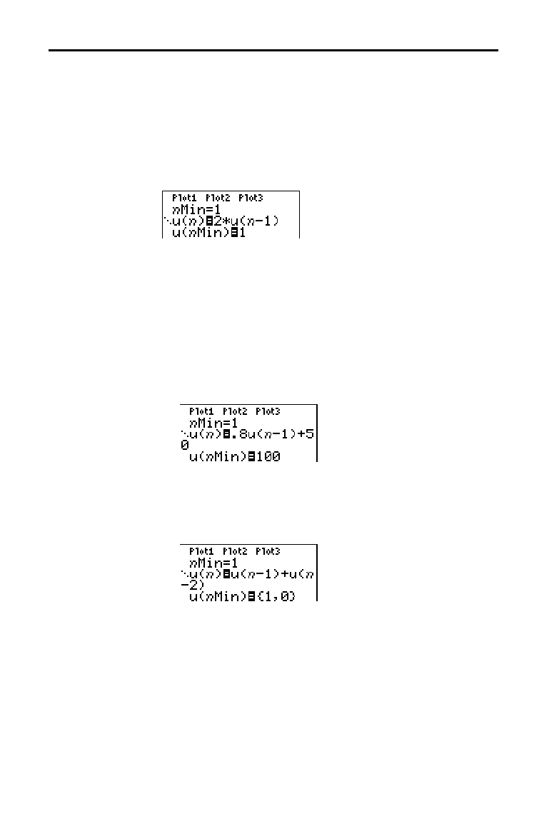
6-6 Sequence Graphing
8306SEQN.DOC TI-83 international English Bob Fedorisko Revised: 02/19/01 12:22 PM Printed: 02/19/01 1:36
PM Page 6 of 16
In a recursive sequence, the
n
th term in the sequence is
defined in relation to the previous term or the term that
precedes the previous term, represented by
u(
n
N
1)
and
u(
n
N
2)
. A recursive sequence may also be defined in
relation to
n
, as in u(
n
)=u(
n
N
1)+
n
.
For example, in the sequence below you cannot calculate
u(5) without first calculating u(1), u(2), u(3), and u(4).
Using an initial value u(
n
Min) = 1, the sequence above
returns
1, 2, 4, 8, 16, . . .
Tip:
On the TI
-
83, you must type each character of the terms. For
example, to enter
u(
n
N
1)
, press
y
[
u
]
£
„
¹
À
¤
.
Recursive sequences require an initial value or values,
since they reference undefined terms.
•
If each term in the sequence is defined in relation to the
previous term, as in
u(
n
N
1)
, you must specify an initial
value for the first term.
•
If each term in the sequence is defined in relation to the
term that precedes the previous term, as in
u(
n
N
2)
, you
must specify initial values for the first two terms. Enter
the initial values as a list enclosed in braces ({ }) with
commas separating the values.
The value of the first term is 0 and the value of the second
term is 1 for the sequence
u(
n
).
Recursive
Sequences

Sequence Graphing 6-7
8306SEQN.DOC TI-83 international English Bob Fedorisko Revised: 02/19/01 12:22 PM Printed: 02/19/01 1:36
PM Page 7 of 16
To display the window variables, press
p
. These
variables define the viewing window. The values below are
defaults for
Seq graphing in both Radian and Degree angle
modes.
nMin=1
Smallest
n
value to evaluate
nMax
=
10
Largest
n
value to evaluate
PlotStart
=
1
First term number to be plotted
PlotStep
=
1
Incremental
n
value (for graphing only)
Xmin
=
L
10
Smallest X value to be displayed
Xmax
=
10
Largest X value to be displayed
Xscl
=
1
Spacing between the X tick marks
Ymin
=
L
10
Smallest Y value to be displayed
Ymax
=
10
Largest Y value to be displayed
Yscl
=
1
Spacing between the Y tick marks
n
Min must be an integer
‚
0.
n
Max, PlotStart, and PlotStep
must be integers
‚
1.
n
Min is the smallest
n
value to evaluate.
n
Min also is
displayed in the sequence
Y=
editor.
n
Max is the largest
n
value to evaluate. Sequences are evaluated at u(
n
Min),
u(
n
Min+1), u(
n
Min+2) , . . . , u(
n
Max).
PlotStart is the first term to be plotted. PlotStart=1 begins
plotting on the first term in the sequence. If you want
plotting to begin with the fifth term in a sequence, for
example, set
PlotStart=5. The first four terms are evaluated
but are not plotted on the graph.
PlotStep is the incremental
n
value for graphing only.
PlotStep does not affect sequence evaluation; it only
designates which points are plotted on the graph. If you
specify
PlotStep=2, the sequence is evaluated at each
consecutive integer, but it is plotted on the graph only at
every other integer.
Setting Window
Variables
6-8 Sequence Graphing
8306SEQN.DOC TI-83 international English Bob Fedorisko Revised: 02/19/01 12:22 PM Printed: 02/19/01 1:36
PM Page 8 of 16
To display the current graph format settings, press
y
[
FORMAT
]. Chapter 3 describes the format settings in detail.
The other graphing modes share these format settings. The
axes setting on the top line of the screen is available only
in
Seq mode.
Time Web uv vw uw
Type of sequence plot (axes)
RectGC PolarGC
Rectangular or polar output
CoordOn CoordOff
Cursor coordinate display on/off
GridOff GridOn
Grid display off or on
AxesOn AxesOff
Axes display on or off
LabelOff LabelOn
Axes label display off or on
ExprOn ExprOff
Expression display on or off
For sequence graphing, you can select from five axes
formats. The table below shows the values that are plotted
on the x-axis and y-axis for each axes setting.
Axes Setting x-axis y-axis
Time
n
u(
n
), v(
n
), w(
n
)
Web u(
n
N
1)
, v(
n
N
1)
, w(
n
N
1) u(
n
), v(
n
), w(
n
)
uv u(
n
)v(
n
)
vw v(
n
)w(
n
)
uw u(
n
)w(
n
)
See pages 6
.
11 and 6
.
12 for more information on Web
plots. See page 6
.
13 for more information on phase plots
(
uv, vw, and uw axes settings).
To plot the selected sequence functions, press
s
. As a
graph is plotted, the TI
-
83 updates
X, Y, and
n
.
Smart Graph applies to sequence graphs (Chapter 3).
Selecting Axes Combinations
Setting the Graph
Format
Setting Axes
Format
Displaying a
Sequence Graph
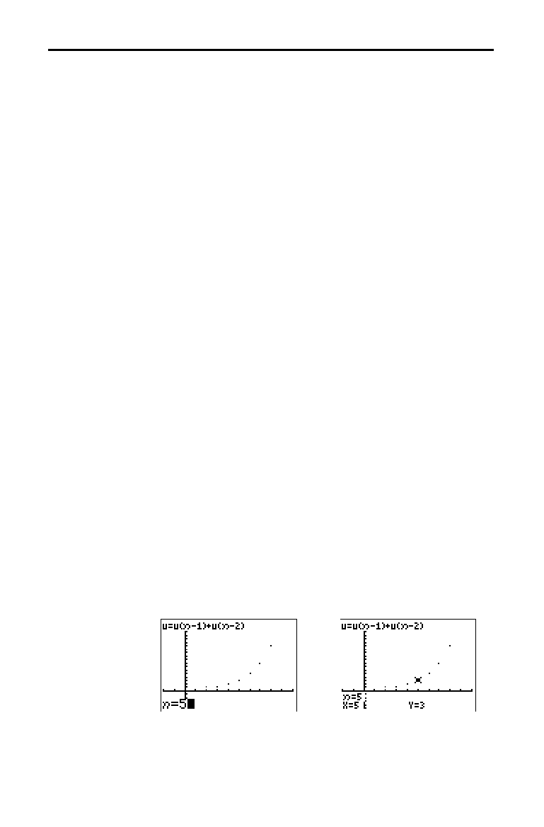
Sequence Graphing 6-9
8306SEQN.DOC TI-83 international English Bob Fedorisko Revised: 02/19/01 12:22 PM Printed: 02/19/01 1:36
PM Page 9 of 16
The free-moving cursor in Seq graphing works the same as
in
Func graphing. In RectGC format, moving the cursor
updates the values of
X and Y; if CoordOn format is
selected,
X and Y are displayed. In PolarGC format, X, Y, R,
and
q
are updated; if CoordOn format is selected, R and
q
are displayed.
The axes format setting affects
TRACE
.
When
Time, uv, vw, or uw axes format is selected,
TRACE
moves the cursor along the sequence one PlotStep
increment at a time. To move five plotted points at once,
press
y
~
or
y
|
.
•
When you begin a trace, the trace cursor is on the first
selected sequence at the term number specified by
PlotStart, even if it is outside the viewing window.
•
Quick Zoom applies to all directions. To center the
viewing window on the current cursor location after
you have moved the trace cursor, press
Í
. The
trace cursor returns to
n
Min.
In
Web format, the trail of the cursor helps identify points
with attracting and repelling behavior in the sequence.
When you begin a trace, the cursor is on the x-axis at the
initial value of the first selected function.
Tip:
To move the cursor to a specified
n
during a trace, enter a value
for
n
, and press
Í
. For example, to quickly return the cursor to the
beginning of the sequence, paste
n
Min
to the
n
=
prompt and press
Í
.
To move the trace cursor to any valid
n
value on the
current function, enter the number. When you enter the
first digit, an
n
= prompt and the number you entered are
displayed in the bottom-left corner of the screen. You can
enter an expression at the
n
= prompt. The value must be
valid for the current viewing window. When you have
completed the entry, press
Í
to move the cursor.
Exploring Sequence Graphs
Free-Moving
Cursor
TRACE
Moving the Trace
Cursor to Any
Valid
n
Value
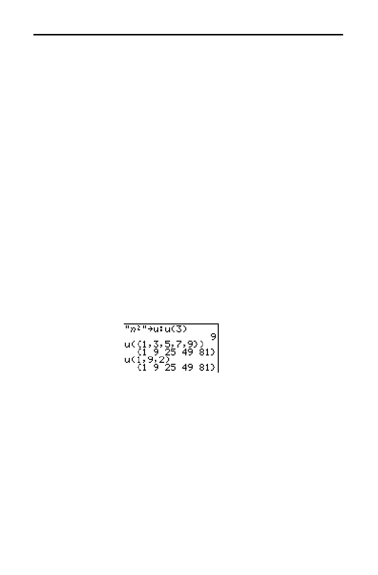
6-10 Sequence Graphing
8306SEQN.DOC TI-83 international English Bob Fedorisko Revised: 02/19/01 12:22 PM Printed: 02/19/01 1:36
PM Page 10 of 16
ZOOM
operations in Seq graphing work the same as in
Func graphing. Only the X (Xmin, Xmax, and Xscl) and Y
(Ymin, Ymax, and Yscl) window variables are affected.
PlotStart, PlotStep,
n
Min, and
n
Max are only affected when
you select
ZStandard. The
VARS Zoom
secondary menu
ZU
items 1 through 7 are the
ZOOM MEMORY
variables for Seq
graphing.
The only
CALC
operation available in Seq graphing is value.
•
When
Time axes format is selected, value displays Y (the
u(
n
) value) for a specified
n
value.
•
When
Web axes format is selected, value draws the web
and displays Y (the u(
n
) value) for a specified
n
value.
•
When
uv, vw, or uw axes format is selected, value
displays X and Y according to the axes format setting.
For example, for uv axes format, X represents u(
n
) and
Y represents v(
n
).
To enter the sequence names
u, v, or w, press
y
[
u
], [
v
], or
[
w
]. You can evaluate these names in any of three ways.
•
Calculate the
n
th value in a sequence.
•
Calculate a list of values in a sequence.
•
Generate a sequence with u(
nstart
,
nstop
[,
nstep
]).
nstep
is optional; default is 1.
ZOOM
CALC
Evaluating u, v,
and w

Sequence Graphing 6-11
8306SEQN.DOC TI-83 international English Bob Fedorisko Revised: 02/19/01 12:22 PM Printed: 02/19/01 1:36
PM Page 11 of 16
To select Web axes format, press
y
[
FORMAT
]
~
Í
. A
web plot graphs
u(
n
) versus u(
n
N
1)
, which you can use to
study long-term behavior (convergence, divergence, or
oscillation) of a recursive sequence. You can see how the
sequence may change behavior as its initial value changes.
When
Web axes format is selected, a sequence will not
graph properly or will generate an error.
•
It must be recursive with only one recursion level
(
u(
n
N
1)
but not u(
n
N
2)
).
•
It cannot reference
n
directly.
•
It cannot reference any defined sequence except itself.
In
Web format, press
s
to display the graph screen.
The TI
-
83:
•
Draws a
y=x
reference line in AxesOn format.
•
Plots the selected sequences with
u(
n
N
1)
as the
independent variable.
Note:
A potential convergence point occurs whenever a sequence
intersects the y=x reference line. However, the sequence may or may
not actually converge at that point, depending on the sequence’s initial
value.
To activate the trace cursor, press
r
. The screen
displays the sequence and the current
n
, X, and Y values (X
represents u(
n
N
1)
and Y represents u(
n
)). Press
~
repeatedly to draw the web step by step, starting at
n
Min.
In
Web format, the trace cursor follows this course.
1. It starts on the x-axis at the initial value
u(
n
Min) (when
PlotStart=1).
2. It moves vertically (up or down) to the sequence.
3. It moves horizontally to the
y=x
reference line.
4. It repeats this vertical and horizontal movement as you
continue to press
~
.
Graphing Web Plots
Graphing a Web
Plot
Valid Functions
for Web Plots
Displaying the
Graph Screen
Drawing the Web
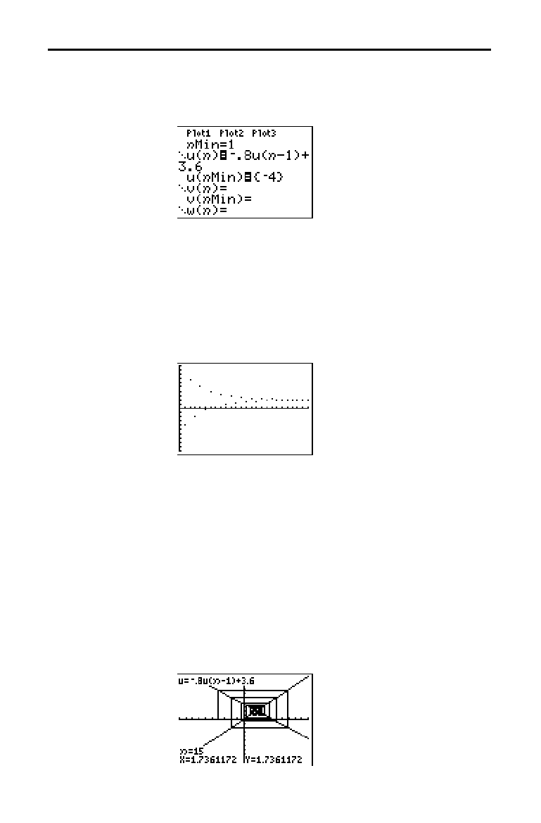
6-12 Sequence Graphing
8306SEQN.DOC TI-83 international English Bob Fedorisko Revised: 02/19/01 12:22 PM Printed: 02/19/01 1:36
PM Page 12 of 16
1. Press
o
in Seq mode to display the sequence
Y=
editor.
Make sure the graph style is set to
í
(dot), and then
define
n
Min, u(
n
) and u(
n
Min) as shown below.
2. Press
y
[
FORMAT
]
Í
to set Time axes format.
3. Press
p
and set the variables as shown below.
n
Min=1 Xmin=0 Ymin=
L
10
n
Max=25 Xmax=25 Ymax=10
PlotStart=1 Xscl=1 Yscl=1
PlotStep=1
4. Press
s
to graph the sequence.
5. Press
y
[
FORMAT
] and select the Web axes setting.
6. Press
p
and change the variables below.
Xmin=
L
10 Xmax=10
7. Press
s
to graph the sequence.
8. Press
r
, and then press
~
to draw the web. The
displayed cursor coordinates
n
, X (u(
n
N
1)
), and
Y (u(
n
)) change accordingly. When you press
~
, a new
n
value is displayed, and the trace cursor is on the
sequence. When you press
~
again, the
n
value remains
the same, and the cursor moves to the
y=x
reference line.
This pattern repeats as you trace the web.
Using Web Plots to Illustrate Convergence
Example:
Convergence
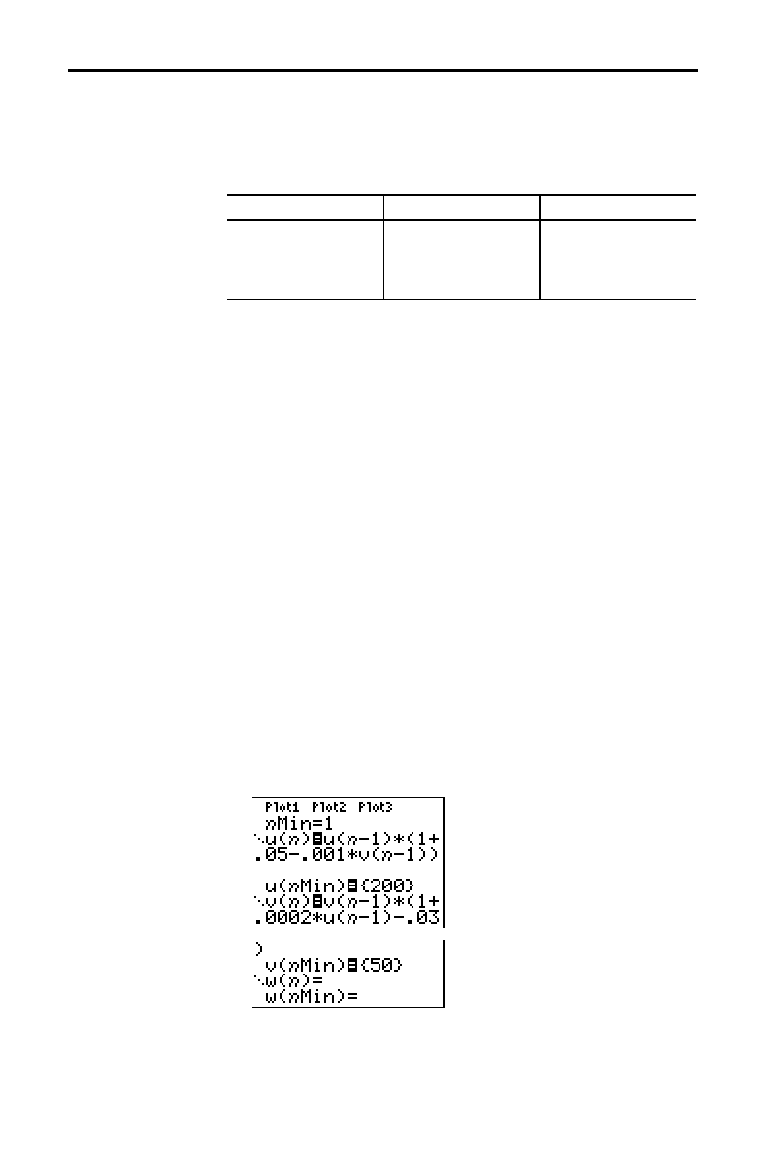
Sequence Graphing 6-13
8306SEQN.DOC TI-83 international English Bob Fedorisko Revised: 02/19/01 12:22 PM Printed: 02/19/01 1:36
PM Page 13 of 16
The phase-plot axes settings uv, vw, and uw show
relationships between two sequences. To select a
phase-plot axes setting, press
y
[
FORMAT
], press
~
until
the cursor is on
uv, vw, or uw, and then press
Í
.
Axes Setting x-axis y-axis
uv u(
n
)v(
n
)
vw v(
n
)w(
n
)
uw u(
n
)w(
n
)
Use the predator-prey model to determine the regional
populations of a predator and its prey that would maintain
population equilibrium for the two species.
This example uses the model to determine the equilibrium
populations of wolves and rabbits, with initial populations
of 200 rabbits (
u(
n
Min)) and 50 wolves (v(
n
Min)).
These are the variables (given values are in parentheses):
R = number of rabbits
M = rabbit population growth rate without wolves (.05)
K = rabbit population death rate with wolves (.001)
W = number of wolves
G = wolf population growth rate with rabbits (.0002)
D = wolf population death rate without rabbits (.03)
n
= time (in months)
R
n
=R
n
N
1
(1+M
N
KW
n
N
1
)
W
n
=W
n
N
1
(1+GR
n
N
1
N
D)
1. Press
o
in
Seq mode to display the sequence
Y=
editor.
Define the sequences and initial values for R
n
and W
n
as
shown below. Enter the sequence R
n
as u(
n
) and enter
the sequence W
n
as v(
n
).
Graphing Phase Plots
Graphing with uv,
vw, and uw
Example:
Predator-Prey
Model
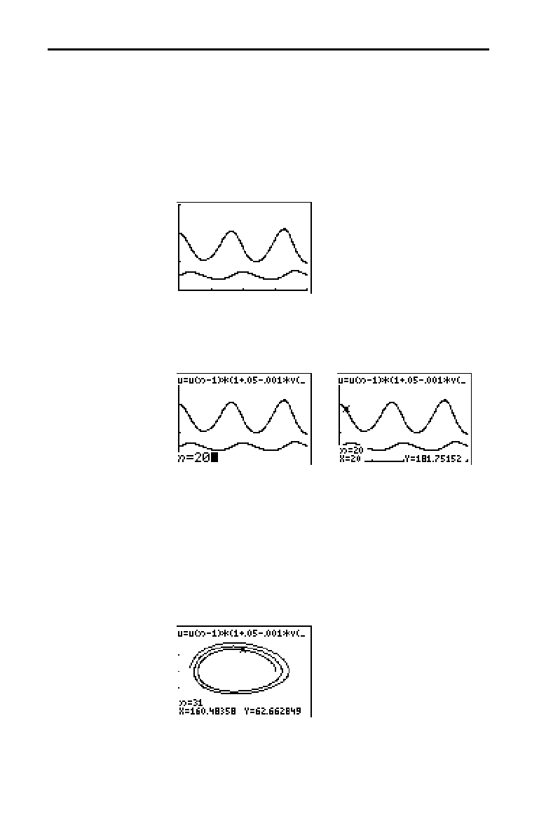
6-14 Sequence Graphing
8306SEQN.DOC TI-83 international English Bob Fedorisko Revised: 02/19/01 12:22 PM Printed: 02/19/01 1:36
PM Page 14 of 16
2. Press
y
[
FORMAT
]
Í
to select Time axes format.
3. Press
p
and set the variables as shown below.
n
Min=0 Xmin=0 Ymin=0
n
Max=400 Xmax=400 Ymax=300
PlotStart=1 Xscl=100 Yscl=100
PlotStep=1
4. Press
s
to graph the sequence.
5. Press
r
~
to individually trace the number of
rabbits (
u(
n
)) and wolves (v(
n
)) over time (
n
).
Tip:
Press a number, and then press
Í
to jump to a specific
n
value (month) while in
TRACE
.
6. Press
y
[
FORMAT
]
~
~
Í
to select uv axes
format.
7. Press
p
and change these variables as shown
below.
Xmin=84 Ymin=25
Xmax=237 Ymax=75
Xscl=50 Yscl=10
8. Press
r
. Trace both the number of rabbits (X) and
the number of wolves (
Y) through 400 generations.
Note:
When you press
r
, the
equation for
u
is displayed in the
top-left corner. Press
}
or
†
to
see the equation for
v
.

Sequence Graphing 6-15
8306SEQN.DOC TI-83 international English Bob Fedorisko Revised: 02/19/01 12:22 PM Printed: 02/19/01 1:36
PM Page 15 of 16
Refer to the table if you are familiar with the TI
-
82. It
shows TI
-
83 sequences and sequence window variables, as
well as their TI
-
82 counterparts.
TI
.
83 TI
.
82
In the
Y=
editor:
u(
n
)U
n
u(
n
Min) U
n
Start
(window variable)
v(
n
)V
n
v(
n
Min) V
n
Start
(window variable)
w(
n
)
not available
w(
n
Min)
not available
In the window editor:
n
Min
n
Start
n
Max
n
Max
PlotStart
n
Min
PlotStep
not available
Comparing TI-83 and TI-82 Sequence Variables
Sequences and
Window
Variables

6-16 Sequence Graphing
8306SEQN.DOC TI-83 international English Bob Fedorisko Revised: 02/19/01 12:22 PM Printed: 02/19/01 1:36
PM Page 16 of 16
Refer to the table if you are familiar with the TI
-
82. It
compares TI
-
83 sequence-name syntax and variable syntax
with TI
.
82 sequence-name syntax and variable syntax.
TI
.
83 / TI
.
82 On TI
.
83, press: On TI
.
82, press:
n
/
n
„y
[
n
]
u(
n
)
/
U
n
y
[
u
]
£
„
¤
y
[
Y
.
VARS
]
¶
À
v(
n
) / V
n
y
[
v
]
£
„
¤
y
[
Y
.
VARS
]
¶
Á
w(
n
)
y
[
w
]
£
„
¤
not available
u(
n
N
1) / U
n
N
1
y
[
u
]
£
„
¹
À
¤
y
[
U
n
N
1
]
v(
n
N
1) / V
n
N
1
y
[
v
]
£
„
¹
À
¤
y
[
V
n
N
1
]
w(
n
N
1)
y
[
w
]
£
„
¹
À
¤
not available
Keystroke Differences Between TI-83 and TI-82
Sequence
Keystroke
Changes
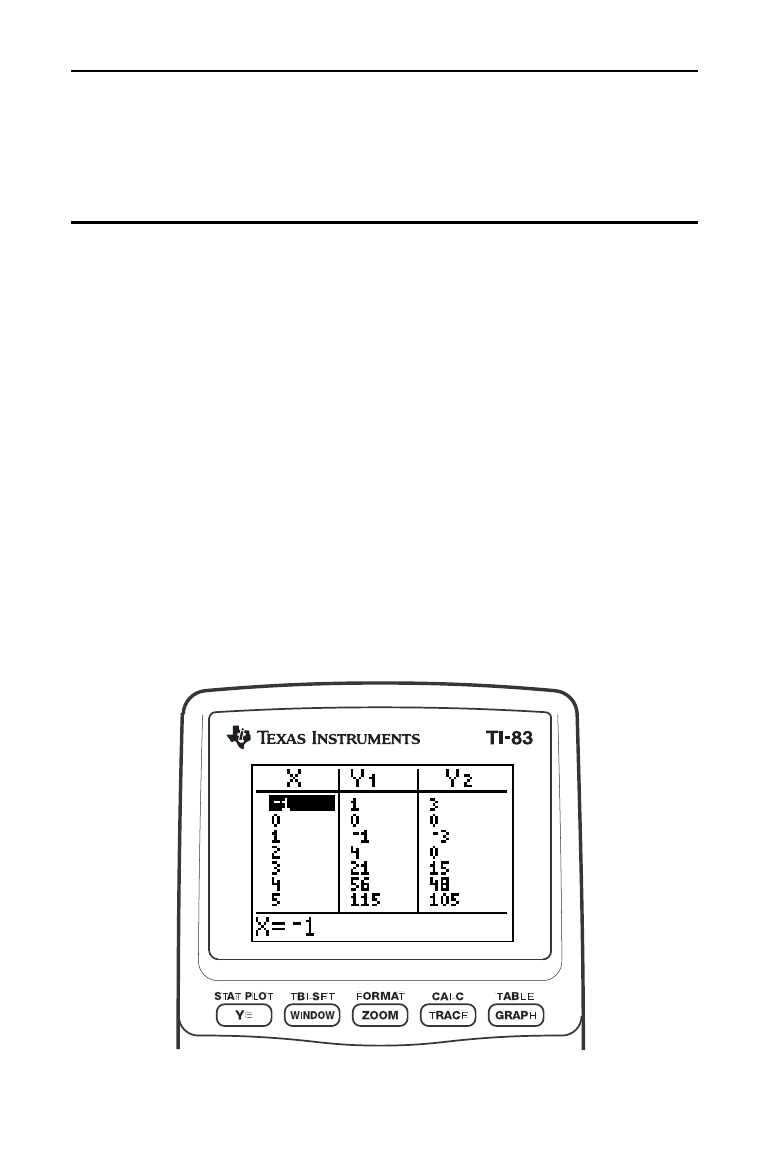
Tables 7-1
8307TABL.DOC TI-83 international English Bob Fedorisko Revised: 02/19/01 12:26 PM Printed: 02/19/01 1:36
PM Page 1 of 6
7
Tables
Getting Started: Roots of a Function
.....................
7-2
Setting Up the Table
.....................................
7-3
Defining the Dependent Variables
........................
7-4
Displaying the Table
.....................................
7-5
Contents
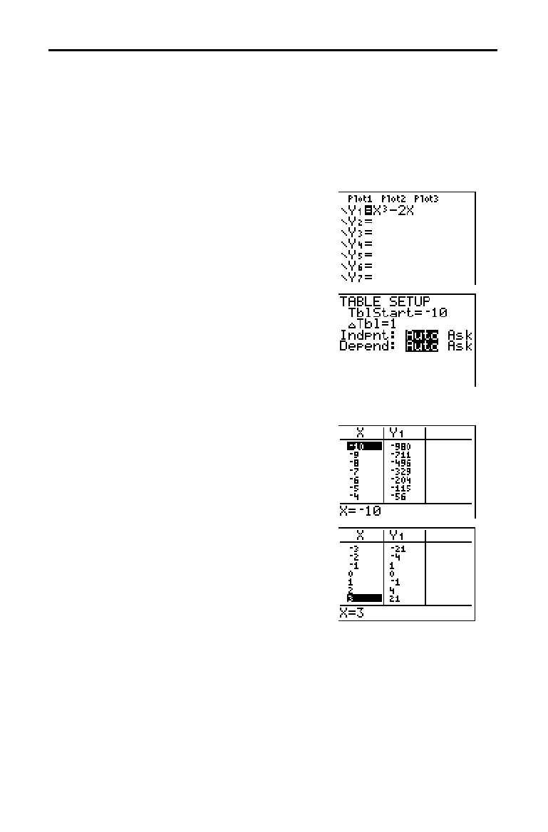
7-2 Tables
8307TABL.DOC TI-83 international English Bob Fedorisko Revised: 02/19/01 12:26 PM Printed: 02/19/01 1:36
PM Page 2 of 6
Getting Started is a fast-paced introduction. Read the chapter for details.
Evaluate the function Y = X
3
N
2X at each integer between
L
10 and 10. How
many sign changes occur, and at what
X values?
1. Press
z
†
†
†
Í
to set
Func
graphing mode.
2. Press
o
. Press
„
3 to select
3
.
Then press
¹
2
„
to enter the
function
Y
1
=X
3
N
2X
.
3. Press
y
[
TBLSET
] to display the
TABLE
SETUP
screen. Press
Ì
10
Í
to set
TblStart=
L
10. Press 1
Í
to set
@
Tbl=1
.
Press
Í
to select
Indpnt: Auto
(automatically generated independent
values). Press
†
Í
to select
Depend: Auto (automatically generated
dependent values).
4. Press
y
[
TABLE
] to display the table
screen.
5. Press
†
until you see the sign changes in
the value of
Y
1
. How many sign changes
occur, and at what
X values?
Getting Started: Roots of a Function

Tables 7-3
8307TABL.DOC TI-83 international English Bob Fedorisko Revised: 02/19/01 12:26 PM Printed: 02/19/01 1:36
PM Page 3 of 6
To display the
TABLE SETUP
screen, press
y
[
TBLSET
].
TblStart (table start) defines the initial value for the
independent variable.
TblStart applies only when the
independent variable is generated automatically (when
Indpnt: Auto is selected).
@
Tbl
(table step) defines the increment for the independent
variable.
Note:
In
Seq
mode, both
TblStart
and
@
Tbl
must be integers.
Selections Table Characteristics
Indpnt: Auto
Depend: Auto
Values are displayed automatically in both
the independent-variable column and in all
dependent-variable columns.
Indpnt: Ask
Depend: Auto
The table is empty; when you enter a value
for the independent variable, all
correspondin
g
dependent-variable values
are calculated and displayed automatically.
Indpnt: Auto
Depend: Ask
Values are displayed automatically for the
independent variable; to
g
enerate a value
for a dependent variable, move the cursor
to that cell and press
Í
.
Indpnt: Ask
Depend: Ask
The table is empty; enter values for the
independent variable; to
g
enerate a value
for a dependent variable, move the cursor
to that cell and press
Í
.
To store a value to
TblStart,
@
Tbl
, or Tbl
Z
nput from the
home screen or a program, select the variable name from
the
VARS TABLE
secondary menu. Tbl
Z
nput is a list of
independent-variable values in the current table.
When you press
y
[
TBLSET
] in the program editor, you
can select
IndpntAuto, IndpntAsk, DependAuto, and
DependAsk.
Setting Up the Table
TABLE SETUP
Screen
TblStart,
@
Tbl
Indpnt: Auto,
Indpnt: Ask,
Depend: Auto,
Depend: Ask
Setting Up the
Table from the
Home Screen or
a Program
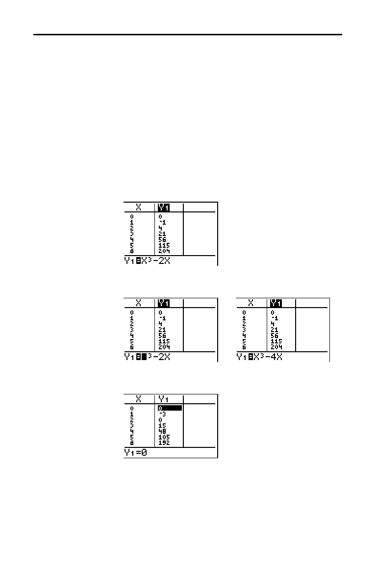
7-4 Tables
8307TABL.DOC TI-83 international English Bob Fedorisko Revised: 02/19/01 12:26 PM Printed: 02/19/01 1:36
PM Page 4 of 6
In the
Y=
editor, enter the functions that define the
dependent variables. Only functions that are selected in the
Y=
editor are displayed in the table. The current graphing
mode is used. In
Par mode, you must define both
components of each parametric equation (Chapter 4).
To edit a selected
Y=
function from the table editor, follow
these steps.
1. Press
y
[
TABLE
] to display the table, then press
~
or
|
to move the cursor to a dependent-variable column.
2. Press
}
until the cursor is on the function name at the
top of the column. The function is displayed on the
bottom line.
3. Press
Í
. The cursor moves to the bottom line. Edit
the function.
4. Press
Í
or
†
. The new values are calculated. The
table and the
Y=
function are updated automatically.
Note:
You also can use this feature to view the function that
defines a dependent variable without having to leave the table.
Defining the Dependent Variables
Defining
Dependent
Variables from
the Y= Editor
Editing
Dependent
Variables from
the Table Editor
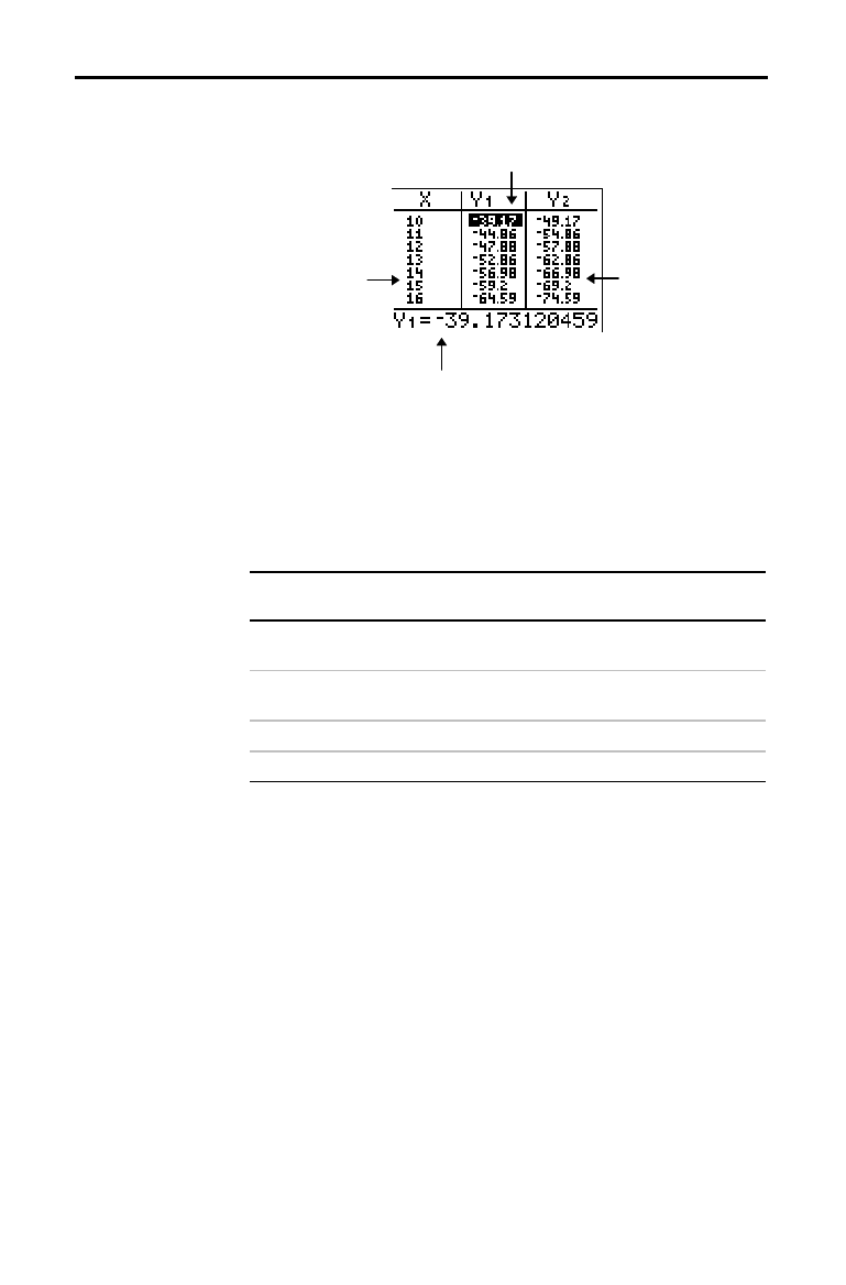
Tables 7-5
8307TABL.DOC TI-83 international English Bob Fedorisko Revised: 02/19/01 12:26 PM Printed: 02/19/01 1:36
PM Page 5 of 6
To display the table, press
y
[
TABLE
].
Current cell
Independent-
variable values
in the first
column
Dependent-
variable values in
the second and
third columns
Current cell’s full value
Note:
The table abbreviates the values, if necessary.
The current graphing mode determines which independent
and dependent variables are displayed in the table
(Chapter 1). In the table above, for example, the
independent variable
X
and the dependent variables
Y
1
and
Y
2
are displayed because
Func
graphing mode is set.
Graphing Mode Independent
Variable
Dependent
Variable
Func
(function)
XY
1
throu
g
h
Y
9
, and
Y
0
Par
(parametric)
TX
1T
/
Y
1T
throu
g
h
X
6T
/
Y
6T
Pol
(polar)
q
r
1
through
r
6
Seq
(sequence)
nu(
n
)
,
v(
n
)
, and
w(
n
)
From the home screen, select the
ClrTable
instruction from
the
CATALOG
. To clear the table, press
Í
.
From a program, select
9:ClrTable
from the
PRGM I/O
menu
or from the
CATALOG
. The table is cleared upon execution.
If
IndpntAsk
is selected, all independent and dependent
variable values on the table are cleared. If
DependAsk
is
selected, all dependent variable values on the table are
cleared.
Displaying the Table
The Table
Independent and
Dependent
Variables
Clearing the
Table from the
Home Screen or
a Program
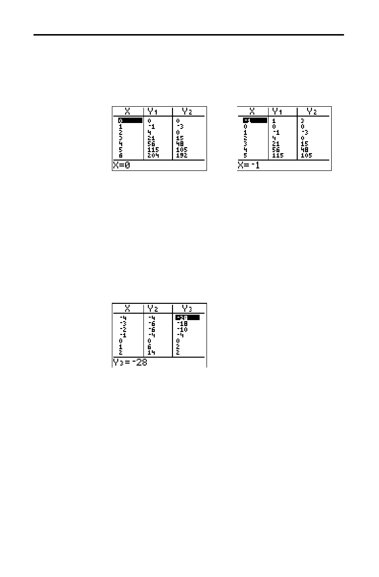
7-6 Tables
8307TABL.DOC TI-83 international English Bob Fedorisko Revised: 02/19/01 12:26 PM Printed: 02/19/01 1:36
PM Page 6 of 6
If Indpnt: Auto is selected, you can press
}
and
†
in the
independent-variable column to display more values. As
you scroll the column, the corresponding dependent-
variable values also are displayed. All dependent-variable
values may not be displayed if
Depend: Ask is selected.
Note:
You can scroll back from the value entered for
TblStart
. As you
scroll,
TblStart
is updated automatically to the value shown on the top
line of the table. In the example above,
TblStart=0
and
@
Tbl=1
generates and displays values of
X=0
, . . . ,
6
; but you can press
}
to
scroll back and display the table for
X=
M
1
, . . .,
5
.
If you have defined more than two dependent variables,
the first two selected
Y=
functions are displayed initially.
Press
~
or
|
to display dependent variables defined by
other selected
Y=
functions. The independent variable
always remains in the left column, except during a trace
with
Par graphing mode and G
.
T split-screen mode set.
Tip:
To simultaneously display on the table two dependent variables
that are not defined as consecutive Y= functions, go to the Y= editor
and deselect the Y= functions between the two you want to display.
For example, to simultaneously display
Y
4
and
Y
7
on the table, go to
the Y= editor and deselect
Y
5
and
Y
6
.
Scrolling
Independent-
Variable Values
Displaying Other
Dependent
Variables

DRAW Instructions 8-1
8308DRAW.DOC TI-83 international English Bob Fedorisko Revised: 02/19/01 12:29 PM Printed: 02/19/01 1:49
PM Page 1 of 20
8
Draw
Instructions
Getting Started: Drawing a Tangent Line
.................
8-2
Using the
DRAW
Menu
...................................
8-3
Clearing Drawings
.......................................
8-4
Drawing Line Segments
..................................
8-5
Drawing Horizontal and Vertical Lines
...................
8-6
Drawing Tangent Lines
..................................
8-8
Drawing Functions and Inverses
.........................
8-9
Shading Areas on a Graph
...............................
8-10
Drawing Circles
..........................................
8-11
Placing Text on a Graph
.................................
8-12
Using Pen to Draw on a Graph
...........................
8-13
Drawing Points on a Graph
..............................
8-14
Drawing Pixels
..........................................
8-16
Storing Graph Pictures (
Pic
s)
............................
8-17
Recalling Graph Pictures (
Pic
s)
..........................
8-18
Storing Graph Databases (
GDB
s)
........................
8-19
Recalling Graph Databases (
GDB
s)
......................
8-20
Contents
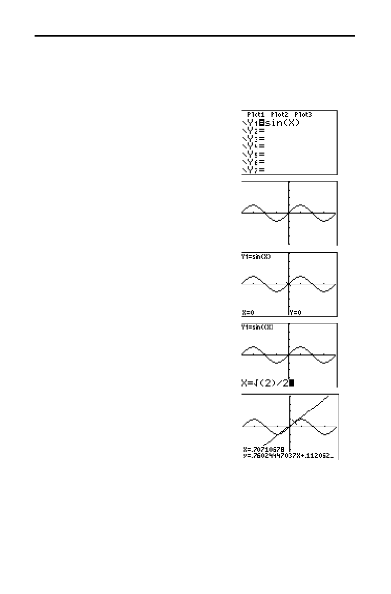
8-2 DRAW Instructions
8308DRAW.DOC TI-83 international English Bob Fedorisko Revised: 02/19/01 12:29 PM Printed: 02/19/01 1:49
PM Page 2 of 20
Getting Started is a fast-paced introduction. Read the chapter for details.
Suppose you want to find the equation of the tangent line at X =
‡
2/2 for the
function Y = sinX.
Before you begin, select
Radian and Func
mode from the mode screen, if necessary.
1. Press
o
to display the
Y=
editor. Press
˜
„
¤
to store
sin(X) in Y
1
.
2. Press
q
7 to select 7:ZTrig, which
graphs the equation in the Zoom Trig
window.
3. Press
y
[
DRAW
] 5 to select 5:Tangent(.
The tangent instruction is initiated.
4. Press
y
[
‡
] 2
¤
¥
2.
5. Press
Í
. The tangent line is drawn; the
X value and the tangent-line equation are
displayed on the graph.
Getting Started: Drawing a Tangent Line

DRAW Instructions 8-3
8308DRAW.DOC TI-83 international English Bob Fedorisko Revised: 02/19/01 12:29 PM Printed: 02/19/01 1:49
PM Page 3 of 20
To display the
DRAW
menu, press
y
[
DRAW
]. The TI
-
83’s
interpretation of these instructions depends on whether
you accessed the menu from the home screen or the
program editor or directly from a graph.
DRAW POINTS STO
1: ClrDraw
Clears all drawn elements.
2: Line(
Draws a line segment between 2 points.
3: Horizontal
Draws a horizontal line.
4: Vertical
Draws a vertical line.
5: Tangent(
Draws a line segment tangent to a function.
6: DrawF
Draws a function.
7: Shade(
Shades an area between two functions.
8: DrawInv
Draws the inverse of a function.
9: Circle(
Draws a circle.
0: Text(
Draws text on a graph screen.
A: Pen
Activates the free-form drawing tool.
The
DRAW
instructions draw on top of graphs. Therefore,
before you use the
DRAW
instructions, consider whether
you want to perform one or more of the following actions.
•
Change the mode settings on the mode screen.
•
Change the format settings on the format screen.
•
Enter or edit functions in the
Y=
editor.
•
Select or deselect functions in the
Y=
editor.
•
Change the window variable values.
•
Turn stat plots on or off.
•
Clear existing drawings with
ClrDraw (page 8
.
4).
Note:
If you draw on a graph and then perform any of the actions
listed above, the graph is replotted without the drawings when you
display the graph again.
You can use any
DRAW
menu instructions except DrawInv
to draw on Func, Par, Pol, and Seq graphs. DrawInv is valid
only in
Func graphing. The coordinates for all
DRAW
instructions are the display’s x-coordinate and y-coordinate
values.
You can use most
DRAW
menu and
DRAW POINTS
menu
instructions to draw directly on a graph, using the cursor
to identify the coordinates. You also can execute these
instructions from the home screen or from within a
program. If a graph is not displayed when you select a
DRAW
menu instruction, the home screen is displayed.
Using the DRAW Menu
DRAW Menu
Before Drawing
on a Graph
Drawing on a
Graph
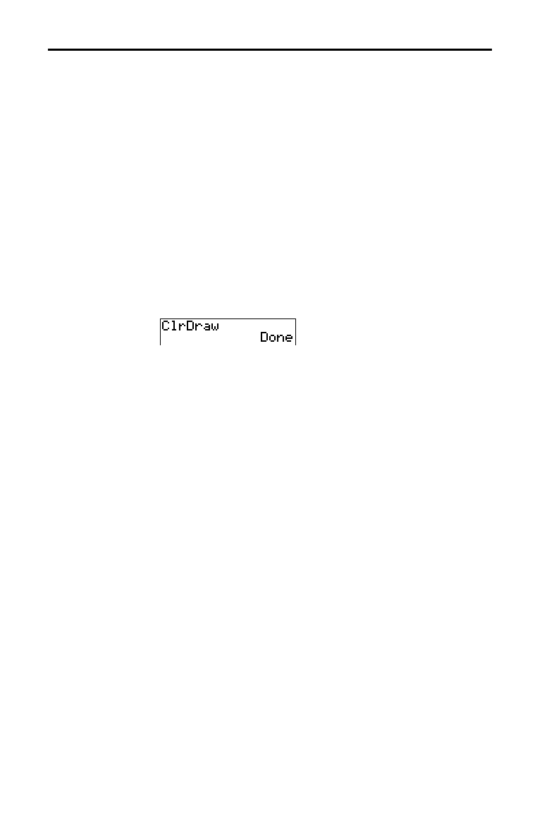
8-4 DRAW Instructions
8308DRAW.DOC TI-83 international English Bob Fedorisko Revised: 02/19/01 12:29 PM Printed: 02/19/01 1:49
PM Page 4 of 20
All points, lines, and shading drawn on a graph with
DRAW
instructions are temporary.
To clear drawings from the currently displayed graph,
select
1:ClrDraw from the
DRAW
menu. The current graph
is replotted and displayed with no drawn elements.
To clear drawings on a graph from the home screen or a
program, begin on a blank line on the home screen or in
the program editor. Select
1:ClrDraw from the
DRAW
menu.
The instruction is copied to the cursor location. Press
Í
.
When
ClrDraw is executed, it clears all drawings from the
current graph and displays the message
Done. When you
display the graph again, all drawn points, lines, circles, and
shaded areas will be gone.
Note:
Before you clear drawings, you can store them with
StorePic
(page 8
.
17).
Clearing Drawings
Clearing
Drawings When
a Graph Is
Displayed
Clearing
Drawings from
the Home Screen
or a Program
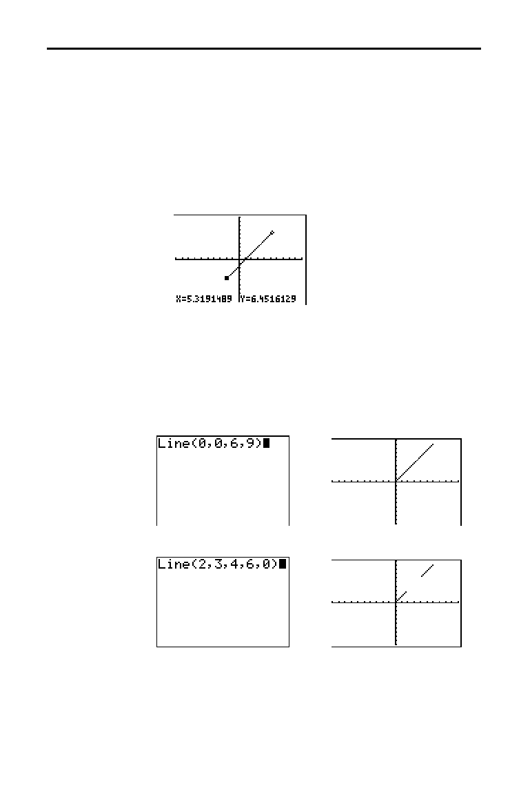
DRAW Instructions 8-5
8308DRAW.DOC TI-83 international English Bob Fedorisko Revised: 02/19/01 12:29 PM Printed: 02/19/01 1:49
PM Page 5 of 20
To draw a line segment when a graph is displayed, follow
these steps.
1. Select
2:Line( from the
DRAW
menu.
2. Place the cursor on the point where you want the line
segment to begin, and then press
Í
.
3. Move the cursor to the point where you want the line
segment to end. The line is displayed as you move the
cursor. Press
Í
.
To continue drawing line segments, repeat steps 2 and 3.
To cancel
Line(, press
‘
.
Line( also draws a line segment between the coordinates
(
X1
,
Y1
) and (
X2
,
Y2
). The values may be entered as
expressions.
Line(
X1
,
Y1
,
X2
,
Y2
)
To erase a line segment, enter Line(
X1
,
Y1
,
X2
,
Y2
,0)
Drawing Line Segments
Drawing a Line
Segment Directly
on a Graph
Drawing a Line
Segment from
the Home Screen
or a Program
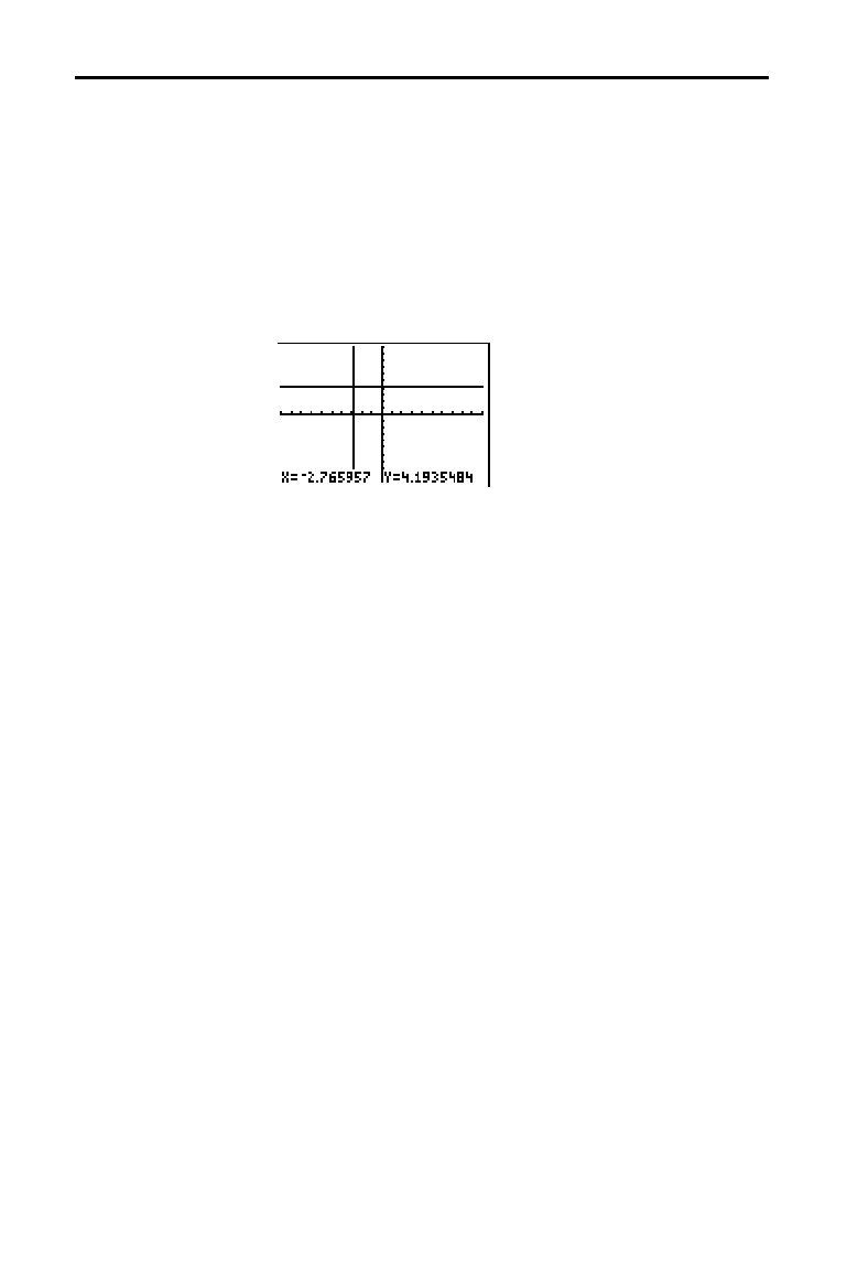
8-6 DRAW Instructions
8308DRAW.DOC TI-83 international English Bob Fedorisko Revised: 02/19/01 12:29 PM Printed: 02/19/01 1:49
PM Page 6 of 20
To draw a horizontal or vertical line when a graph is
displayed, follow these steps.
1. Select
3:Horizontal or 4:Vertical from the
DRAW
menu. A
line is displayed that moves as you move the cursor.
2. Place the cursor on the y-coordinate (for horizontal
lines) or x-coordinate (for vertical lines) through which
you want the drawn line to pass.
3. Press
Í
to draw the line on the graph.
To continue drawing lines, repeat steps 2 and 3.
To cancel
Horizontal or Vertical, press
‘
.
Drawing Horizontal and Vertical Lines
Drawing a Line
Directly on a
Graph
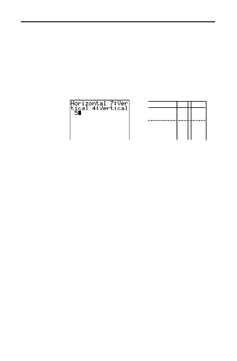
DRAW Instructions 8-7
8308DRAW.DOC TI-83 international English Bob Fedorisko Revised: 02/19/01 12:29 PM Printed: 02/19/01 1:49
PM Page 7 of 20
Horizontal (horizontal line) draws a horizontal line at Y=
y
.
y
can be an expression but not a list.
Horizontal
y
Vertical (vertical line) draws a vertical line at X=
x
.
x
can be
an expression but not a list.
Vertical
x
To instruct the TI
-
83 to draw more than one horizontal or
vertical line, separate each instruction with a colon (
: ).
Drawing a Line
from the Home
Screen or a
Program
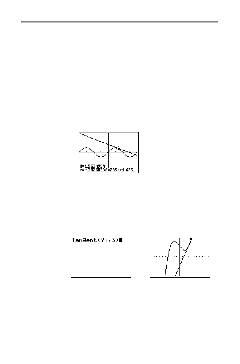
8-8 DRAW Instructions
8308DRAW.DOC TI-83 international English Bob Fedorisko Revised: 02/19/01 12:29 PM Printed: 02/19/01 1:49
PM Page 8 of 20
To draw a tangent line when a graph is displayed, follow
these steps.
1. Select
5:Tangent( from the
DRAW
menu.
2. Press
†
and
}
to move the cursor to the function for
which you want to draw the tangent line. The current
graph’s
Y=
function is displayed in the top-left corner, if
ExprOn is selected.
3. Press
~
and
|
or enter a number to select the point on
the function at which you want to draw the tangent line.
4. Press
Í
. In
Func mode, the X value at which the
tangent line was drawn is displayed on the bottom of
the screen, along with the equation of the tangent line.
In all other modes, the
dy/dx value is displayed.
Tip:
Change the fixed decimal setting on the mode screen if you want
to see fewer digits displayed for
X
and the equation for
Y
.
Tangent( (tangent line) draws a line tangent to
expression
in terms of
X, such as Y
1
or X
2
, at point X=
value
.
X can be
an expression.
expression
is interpreted as being in
Func
mode.
Tangent(
expression
,
value
)
Drawing Tangent Lines
Drawing
a Tangent Line
Directly
on a Graph
Drawing
a Tangent Line
from the Home
Screen or
a Program
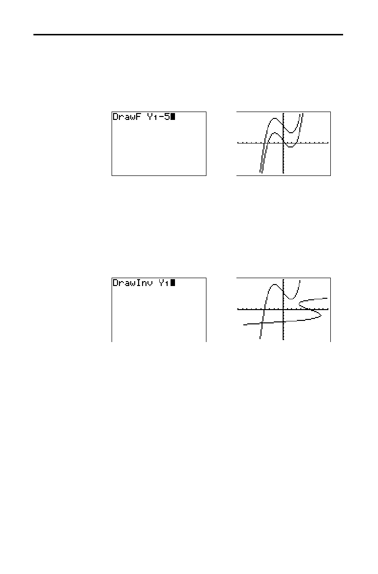
DRAW Instructions 8-9
8308DRAW.DOC TI-83 international English Bob Fedorisko Revised: 02/19/01 12:29 PM Printed: 02/19/01 1:49
PM Page 9 of 20
DrawF (draw function) draws
expression
as a function in
terms of
X on the current graph. When you select 6:DrawF
from the
DRAW
menu, the TI
-
83 returns to the home screen
or the program editor.
DrawF is not interactive.
DrawF
expression
Note:
You cannot use a list in
expression
to draw a family of curves.
DrawInv (draw inverse) draws the inverse of
expression
by
plotting
X values on the y-axis and Y values on the x-axis.
When you select
8:DrawInv from the
DRAW
menu, the TI
-
83
returns to the home screen or the program editor.
DrawInv
is not interactive. DrawInv works in Func mode only.
DrawInv
expression
Note:
You cannot use a list in
expression
to draw a family of curves.
Drawing Functions and Inverses
Drawing a
Function
Drawing an
Inverse of a
Function
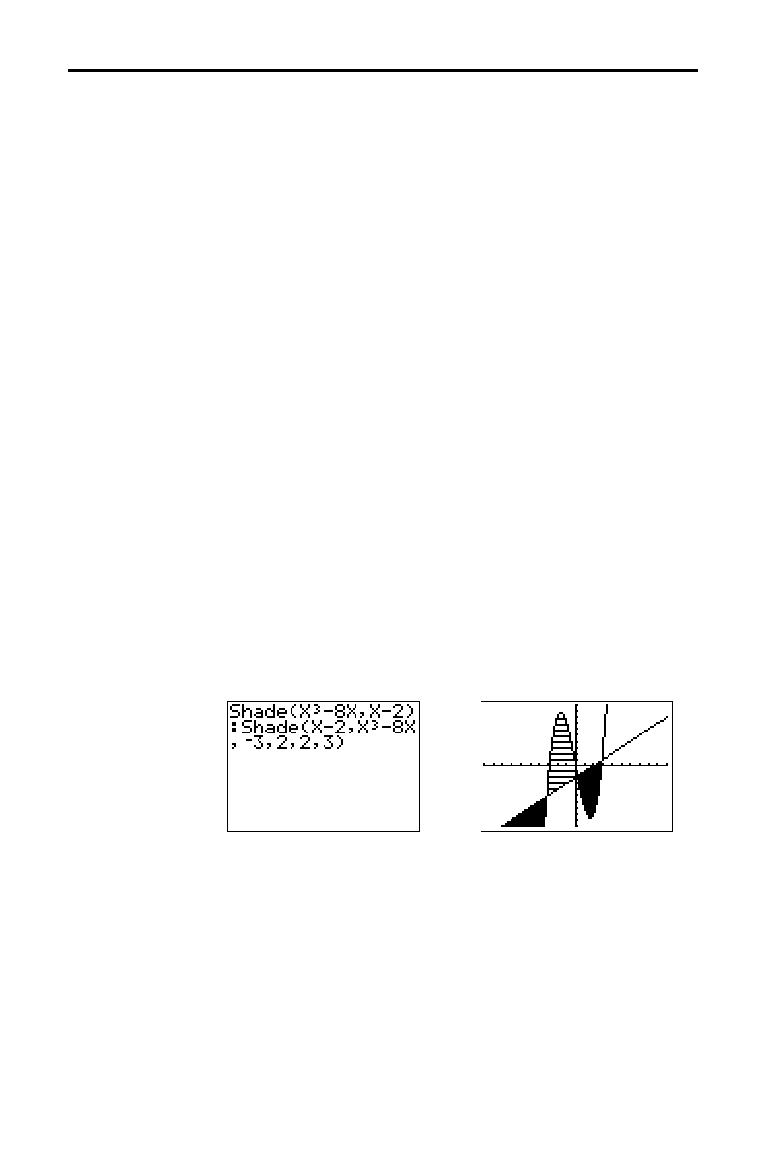
8-10 DRAW Instructions
8308DRAW.DOC TI-83 international English Bob Fedorisko Revised: 02/19/01 12:29 PM Printed: 02/19/01 1:49
PM Page 10 of 20
To shade an area on a graph, select 7:Shade( from the
DRAW
menu. The instruction is pasted to the home screen
or to the program editor.
Shade( draws
lowerfunc
and
upperfunc
in terms of X on
the current graph and shades the area that is specifically
above
lowerfunc
and below
upperfunc
. Only the areas
where
lowerfunc
<
upperfunc
are shaded.
Xleft
and
Xright
, if included, specify left and right
boundaries for the shading.
Xleft
and
Xright
must be
numbers between
Xmin and Xmax, which are the defaults.
pattern
specifies one of four shading patterns.
pattern=
1 vertical (default)
pattern=
2 horizontal
pattern=
3 negative—slope 45
¡
pattern=
4 positive—slope 45
¡
patres
specifies one of eight shading resolutions.
patres=
1 shades every pixel (default)
patres=
2 shades every second pixel
patres
=
3 shades every third pixel
patres
=
4 shades every fourth pixel
patres
=
5 shades every fifth pixel
patres
=
6 shades every sixth pixel
patres
=
7 shades every seventh pixel
patres
=
8 shades every eighth pixel
Shade(
lowerfunc
,
upperfunc
[
,
Xleft
,
Xright
,
pattern
,
patres
]
)
Shading Areas on a Graph
Shading a Graph
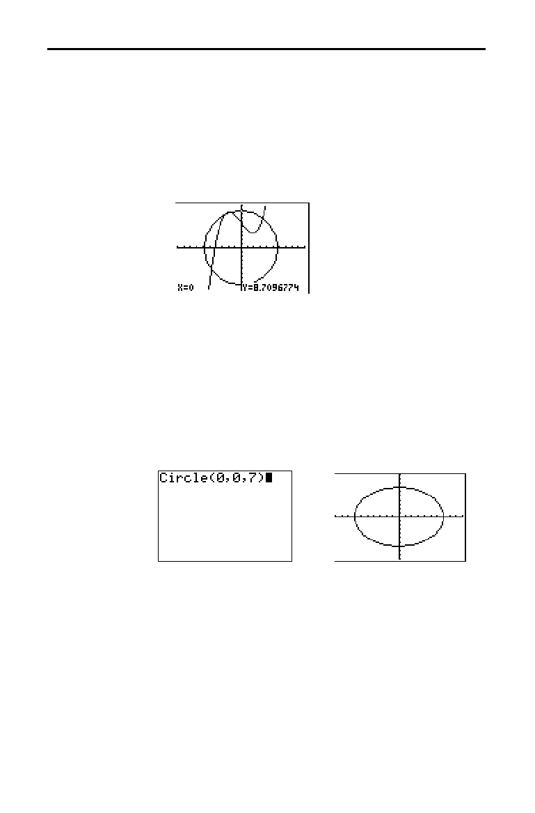
DRAW Instructions 8-11
8308DRAW.DOC TI-83 international English Bob Fedorisko Revised: 02/19/01 12:29 PM Printed: 02/19/01 1:49
PM Page 11 of 20
To draw a circle directly on a displayed graph using the
cursor, follow these steps.
1. Select
9:Circle( from the
DRAW
menu.
2. Place the cursor at the center of the circle you want to
draw. Press
Í
.
3. Move the cursor to a point on the circumference. Press
Í
to draw the circle on the graph.
Note:
This circle is displayed as circular, regardless of the window
variable values, because you drew it directly on the display. When
you use the
Circle(
instruction from the home screen or a
program, the current window variables may distort the shape.
To continue drawing circles, repeat steps 2 and 3. To
cancel
Circle(, press
‘
.
Circle( draws a circle with center (
X
,
Y
) and
radius.
These
values can be expressions.
Circle(
X
,
Y
,
radius
)
Tip:
When you use
Circle(
on the home screen or from a program,
the current window values may distort the drawn circle. Use
ZSquare
(Chapter 3) before drawing the circle to adjust the window variables
and make the circle circular.
Drawing Circles
Drawing a Circle
Directly on a
Graph
Drawing a Circle
from the Home
Screen or a
Program
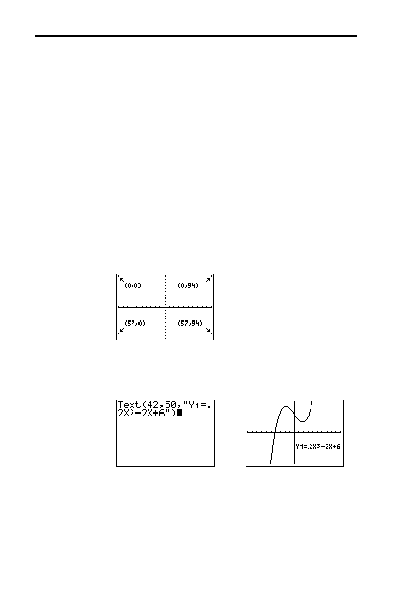
8-12 DRAW Instructions
8308DRAW.DOC TI-83 international English Bob Fedorisko Revised: 02/19/01 12:29 PM Printed: 02/19/01 1:49
PM Page 12 of 20
To place text on a graph when the graph is displayed,
follow these steps.
1. Select
0:Text( from the
DRAW
menu.
2. Place the cursor where you want the text to begin.
3. Enter the characters. Press
ƒ
or
y
[
A
.
LOCK
] to
enter letters and
q
. You may enter TI
-
83 functions,
variables, and instructions. The font is proportional, so
the exact number of characters you can place on the
graph varies. As you type, the characters are placed on
top of the graph.
To cancel
Text(, press
‘
.
Text( places on the current graph the characters
comprising
value
, which can include TI
-
83 functions and
instructions. The top-left corner of the first character is at
pixel (
row
,
column
), where
row
is an integer between
0 and 57 and
column
is an integer between 0 and 94. Both
row
and
column
can be expressions.
Text(
row
,
column
,
value
,
value
. . .
)
value
can be text enclosed in quotation marks (
" ), or it
can be an expression. The TI
-
83 will evaluate an
expression and display the result with up to 10 characters.
On a Horiz split screen, the maximum value for
row
is 25.
On a
G
.
T split screen, the maximum value for
row
is 45,
and the maximum value for
column
is 46.
Placing Text on a Graph
Placing Text
Directly on a
Graph
Placing Text on a
Graph from the
Home Screen or
a Program
Split Screen
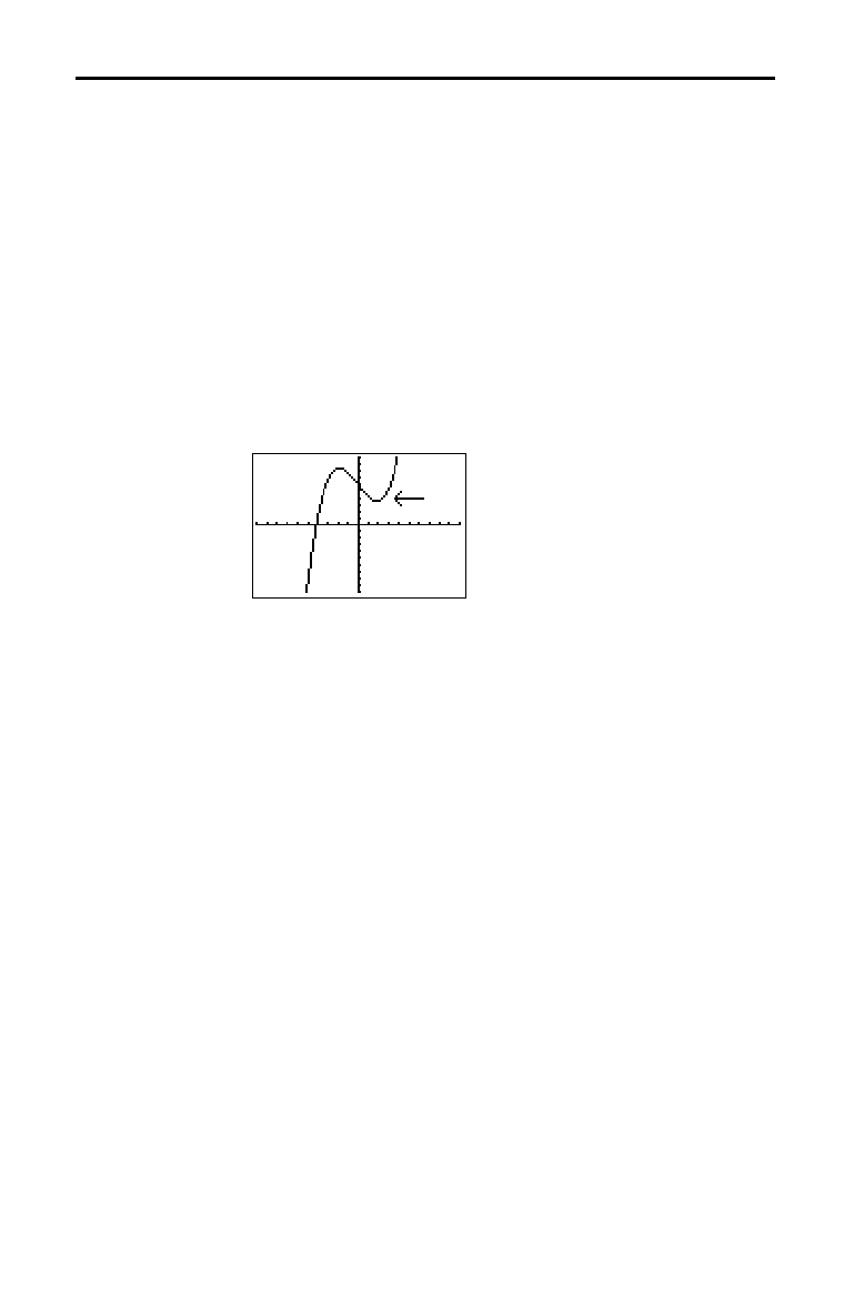
DRAW Instructions 8-13
8308DRAW.DOC TI-83 international English Bob Fedorisko Revised: 02/19/01 12:29 PM Printed: 02/19/01 1:49
PM Page 13 of 20
Pen draws directly on a graph only. You cannot execute
Pen from the home screen or a program.
To draw on a displayed graph, follow these steps.
1. Select
A:Pen from the
DRAW
menu.
2. Place the cursor on the point where you want to begin
drawing. Press
Í
to turn on the pen.
3. Move the cursor. As you move the cursor, you draw on
the graph, shading one pixel at a time.
4. Press
Í
to turn off the pen.
For example,
Pen was used to create the arrow pointing to
the local minimum of the selected function.
To continue drawing on the graph, move the cursor to a
new position where you want to begin drawing again, and
then repeat steps 2, 3, and 4. To cancel
Pen, press
‘
.
Using Pen to Draw on a Graph
Using Pen to
Draw on a Graph
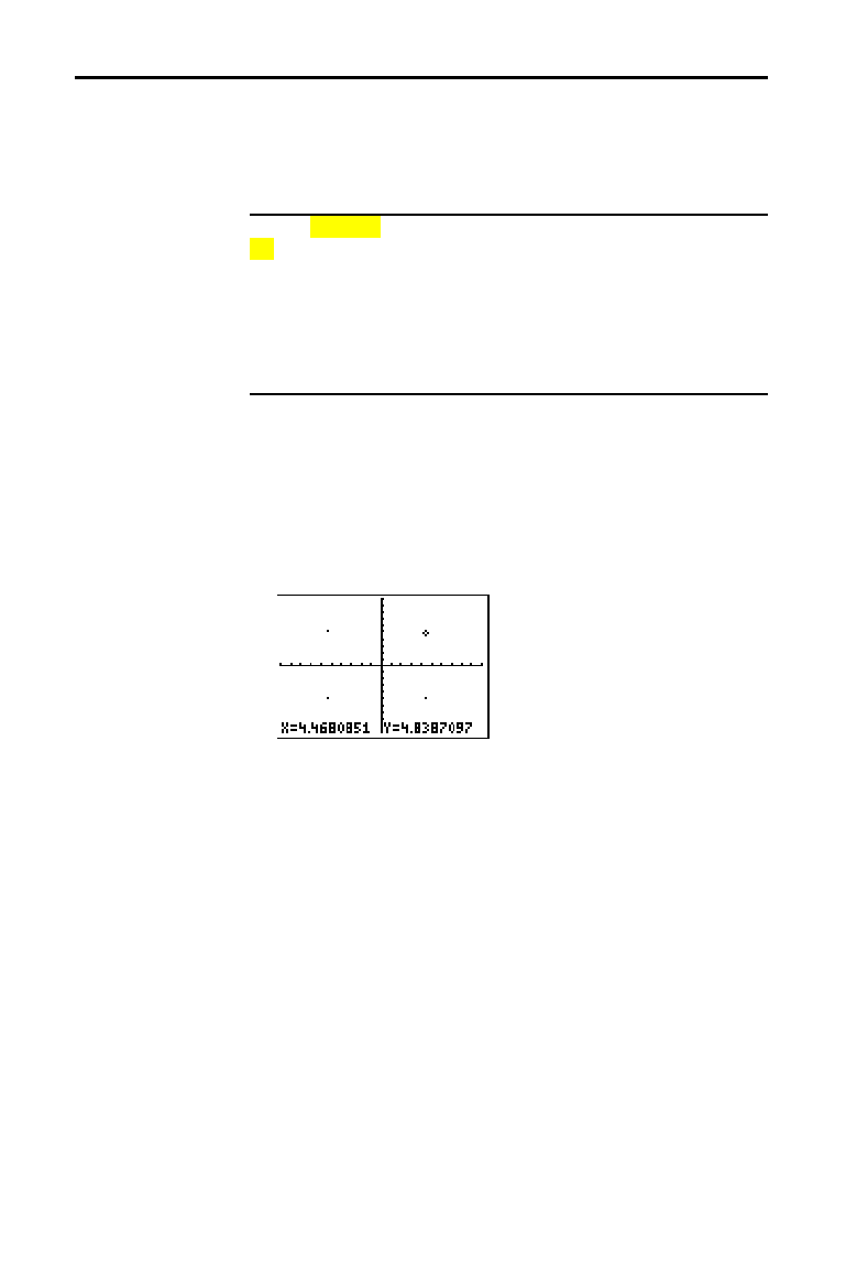
8-14 DRAW Instructions
8308DRAW.DOC TI-83 international English Bob Fedorisko Revised: 02/19/01 12:29 PM Printed: 02/19/01 1:49
PM Page 14 of 20
To display the
DRAW POINTS
menu, press
y
[
DRAW
]
~
.
The TI
-
83’s interpretation of these instructions depends on
whether you accessed this menu from the home screen or
the program editor or directly from a graph.
DRAW POINTS STO
1: Pt-On(
Turns on a point.
2: Pt-Off(
Turns off a point.
3: Pt-Change(
Toggles a point on or off.
4: Pxl-On(
Turns on a pixel.
5: Pxl-Off(
Turns off a pixel.
6: Pxl-Change(
Toggles a pixel on or off.
7: pxl-Test(
Returns 1 if pixel on, 0 if pixel off.
To draw a point on a graph, follow these steps.
1. Select
1:Pt
.
On( from the
DRAW POINTS
menu.
2. Move the cursor to the position where you want to draw
the point.
3. Press
Í
to draw the point.
To continue drawing points, repeat steps 2 and 3. To
cancel
Pt
.
On(, press
‘
.
Drawing Points on a Graph
DRAW POINTS
Menu
Drawing Points
Directly on a
Graph with
Pt
-
On(

DRAW Instructions 8-15
8308DRAW.DOC TI-83 international English Bob Fedorisko Revised: 02/19/01 12:29 PM Printed: 02/19/01 1:49
PM Page 15 of 20
To erase (turn off) a drawn point on a graph, follow these
steps.
1. Select
2:Pt
.
Off( (point off) from the
DRAW POINTS
menu.
2. Move the cursor to the point you want to erase.
3. Press
Í
to erase the point.
To continue erasing points, repeat steps 2 and 3. To cancel
Pt
.
Off(, press
‘
.
To change (toggle on or off) a point on a graph, follow
these steps.
1. Select
3:Pt
.
Change( (point change) from the
DRAW
POINTS
menu.
2. Move the cursor to the point you want to change.
3. Press
Í
to change the point’s on/off status.
To continue changing points, repeat steps 2 and 3. To
cancel
Pt
.
Change(, press
‘
.
Pt
.
On( (point on) turns on the point at (X=
x
,Y=
y
). Pt
.
Off(
turns the point off. Pt
.
Change( toggles the point on or off.
mark
is optional; it determines the point’s appearance;
specify
1, 2, or 3, where:
1 =
¦
(dot; default) 2 =
›
(box) 3 = + (cross)
Pt
.
On(
x
,
y
[
,
mark
]
)
Pt
.
Off(
x
,
y
[
,
mark
]
)
Pt
.
Change(
x
,
y
)
Note:
If you specified
mark
to turn on a point with
Pt
.
On(
, you must
specify
mark
when you turn off the point with
Pt
.
Off(
.
Pt
.
Change(
does not have the
mark
option.
Erasing Points
with Pt-Off(
Changing Points
with Pt-Change(
Drawing Points
from the Home
Screen or a
Program
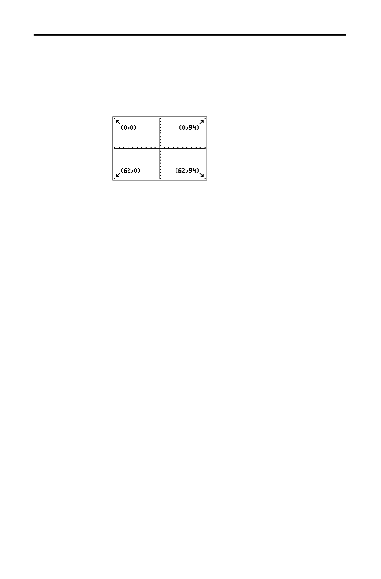
8-16 DRAW Instructions
8308DRAW.DOC TI-83 international English Bob Fedorisko Revised: 02/19/01 12:29 PM Printed: 02/19/01 1:49
PM Page 16 of 20
A pixel is a square dot on the TI
-
83 display. The Pxl
.
(pixel)
instructions let you turn on, turn off, or reverse a pixel
(dot) on the graph using the cursor. When you select a
pixel instruction from the
DRAW POINTS
menu, the TI
-
83
returns to the home screen or the program editor. The
pixel instructions are not interactive.
Pxl
.
On( (pixel on) turns on the pixel at (
row
,
column
),
where
row
is an integer between 0 and 62 and
column
is an
integer between 0 and 94.
Pxl
.
Off( turns the pixel off. Pxl
.
Change( toggles the pixel on
and off.
Pxl
.
On(
row
,
column
)
Pxl
.
Off(
row
,
column
)
Pxl
.
Change(
row
,
column
)
pxl
.
Test(
(pixel test) returns 1 if the pixel at (
row
,
column
)
is turned on or 0 if the pixel is turned off on the current
graph.
row
must be an integer between 0 and 62.
column
must be an integer between 0 and 94.
pxl
.
Test(
row
,
column
)
On a Horiz split screen, the maximum value for
row
is 30
for
Pxl
.
On(, Pxl
.
Off(, Pxl
.
Change(, and pxl
.
Test(.
On a
G
.
T split screen, the maximum value for
row
is 50 and
the maximum value for
column
is 46 for
Pxl
.
On(, Pxl
.
Off(,
Pxl
.
Change(, and pxl
.
Test(.
Drawing Pixels
TI-83 Pixels
Turning On and
Off Pixels with
Pxl-On( and
Pxl-Off(
Using pxl-Test(
Split Screen
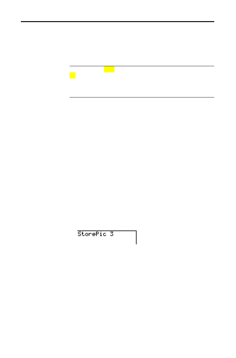
DRAW Instructions 8-17
8308DRAW.DOC TI-83 international English Bob Fedorisko Revised: 02/19/01 12:29 PM Printed: 02/19/01 1:49
PM Page 17 of 20
To display the
DRAW STO
menu, press
y
[
DRAW
]
|
.
When you select an instruction from the
DRAW STO
menu,
the TI
-
83 returns to the home screen or the program editor.
The picture and graph database instructions are not
interactive.
DRAW POINTS STO
1:StorePic
Stores the current picture.
2:RecallPic
Recalls a saved picture.
3:StoreGDB
Stores the current graph database.
4:RecallGDB
Recalls a saved graph database.
You can store up to 10 graph pictures, each of which is an
image of the current graph display, in picture variables
Pic1 through Pic9, or Pic0. Later, you can superimpose the
stored picture onto a displayed graph from the home
screen or a program.
A picture includes drawn elements, plotted functions, axes,
and tick marks. The picture does not include axes labels,
lower and upper bound indicators, prompts, or cursor
coordinates. Any parts of the display hidden by these items
are stored with the picture.
To store a graph picture, follow these steps.
1. Select
1:StorePic from the
DRAW STO
menu. StorePic is
pasted to the current cursor location.
2. Enter the number (from
1 to 9, or 0) of the picture
variable to which you want to store the picture. For
example, if you enter
3, the TI
-
83 will store the picture
to
Pic3.
Note:
You also can select a variable from the
PICTURE
secondary menu (
4
). The variable is pasted next to
StorePic
.
3. Press
Í
to display the current graph and store the
picture.
Storing Graph Pictures (Pics)
DRAW STO Menu
Storing a Graph
Picture
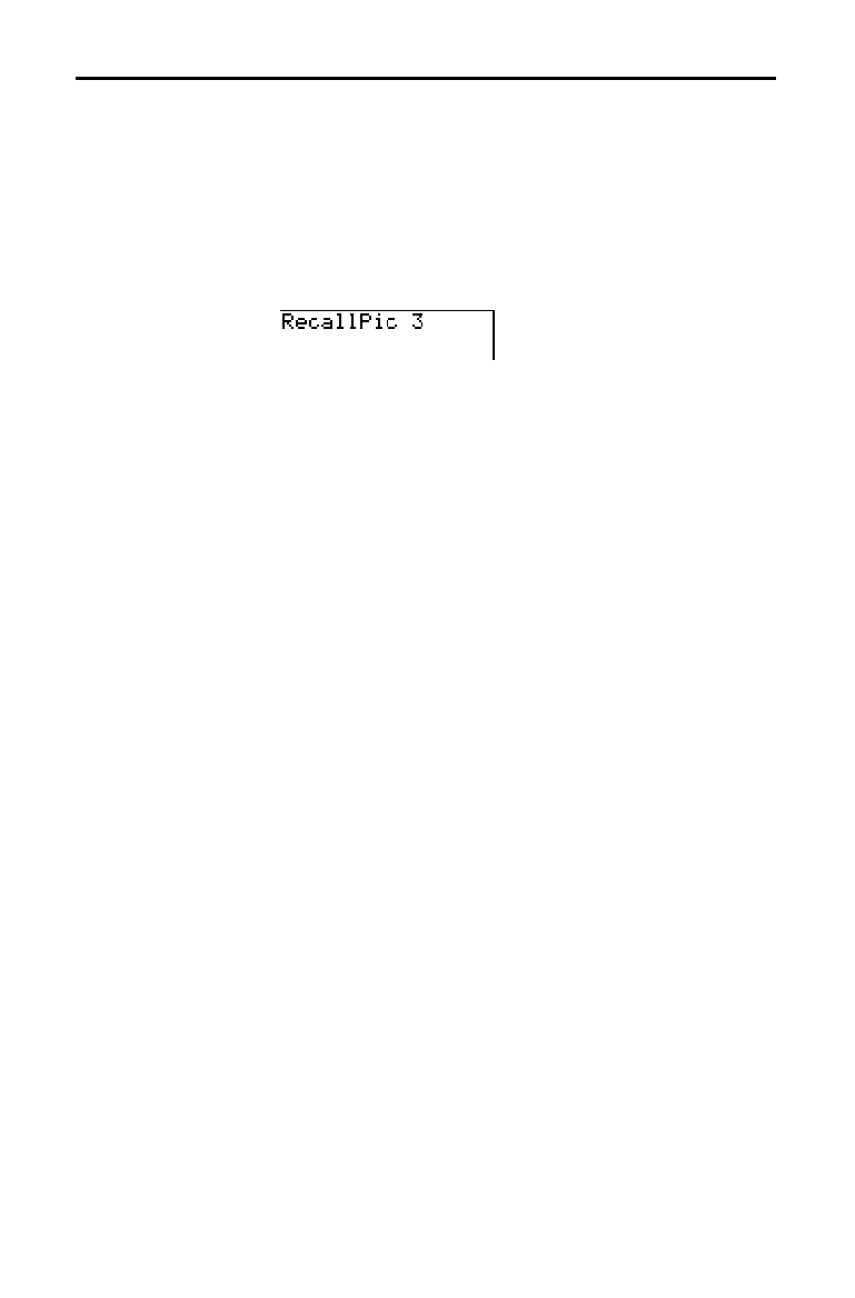
8-18 DRAW Instructions
8308DRAW.DOC TI-83 international English Bob Fedorisko Revised: 02/19/01 12:29 PM Printed: 02/19/01 1:49
PM Page 18 of 20
To recall a graph picture, follow these steps.
1. Select
2:RecallPic from the
DRAW STO
menu. RecallPic
is pasted to the current cursor location.
2. Enter the number (from
1 to 9, or 0) of the picture
variable from which you want to recall a picture. For
example, if you enter
3, the TI
-
83 will recall the picture
stored to
Pic3.
Note:
You also can select a variable from the
PICTURE
secondary menu (
4
). The variable is pasted next to
RecallPic
.
3. Press
Í
to display the current graph with the
picture superimposed on it.
Note:
Pictures are drawings. You cannot trace a curve that is part of a
picture.
To delete graph pictures from memory, use the
MEMORY DELETE FROM
menu (Chapter 18).
Recalling Graph Pictures (Pics)
Recalling a
Graph Picture
Deleting a Graph
Picture

DRAW Instructions 8-19
8308DRAW.DOC TI-83 international English Bob Fedorisko Revised: 02/19/01 12:29 PM Printed: 02/19/01 1:49
PM Page 19 of 20
A graph database (
GDB
) contains the set of elements that
defines a particular graph. You can recreate the graph from
these elements. You can store up to 10
GDB
s in variables
GDB1 through GDB9, or GDB0 and recall them to recreate
graphs.
A
GDB
stores five elements of a graph.
•
Graphing mode
•
Window variables
•
Format settings
•
All functions in the
Y=
editor and the selection status of
each
•
Graph style for each
Y=
function
GDB
s do not contain drawn items or stat plot definitions.
To store a graph database, follow these steps.
1. Select
3:StoreGDB from the
DRAW STO
menu. StoreGDB
is pasted to the current cursor location.
2. Enter the number (from
1 to 9, or 0) of the
GDB
variable
to which you want to store the graph database. For
example, if you enter
7, the TI
-
83 will store the
GDB
to
GDB7.
Note:
You also can select a variable from the
GDB
secondary
menu (
3
). The variable is pasted next to
StoreGDB
.
3. Press
Í
to store the current database to the
specified
GDB
variable.
Storing Graph Databases (GDBs)
What Is a Graph
Database?
Storing a Graph
Database
8-20 DRAW Instructions
8308DRAW.DOC TI-83 international English Bob Fedorisko Revised: 02/19/01 12:29 PM Printed: 02/19/01 1:49
PM Page 20 of 20
CAUTION:
When you recall a
GDB
, it replaces all existing
Y=
functions. Consider storing the current
Y=
functions to
another database before recalling a stored
GDB
.
To recall a graph database, follow these steps.
1. Select
4:RecallGDB from the
DRAW STO
menu.
RecallGDB is pasted to the current cursor location.
2. Enter the number (from
1 to 9, or 0) of the
GDB
variable
from which you want to recall a
GDB
. For example, if
you enter
7, the TI
-
83 will recall the
GDB
stored to
GDB7.
Note:
You also can select a variable from the
GDB
secondary
menu (
3
). The variable is pasted next to
RecallGDB
.
3. Press
Í
to replace the current
GDB
with the
recalled
GDB
. The new graph is not plotted. The TI
-
83
changes the graphing mode automatically, if necessary.
To delete a
GDB
from memory, use the
MEMORY DELETE
FROM
menu (Chapter 18).
Recalling Graph Databases (GDBs)
Recalling a
Graph Database
Deleting a Graph
Database
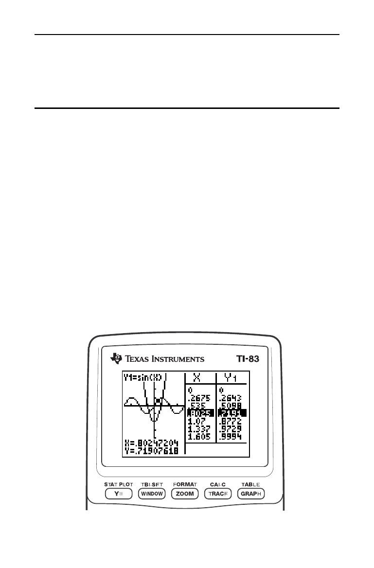
Split Screen 9-1
8309SPLT.DOC TI-83 international English Bob Fedorisko Revised: 02/19/01 12:31 PM Printed: 02/19/01 1:36
PM Page 1 of 6
9
Split
Screen
Getting Started: Exploring the Unit Circle
................
9-2
Using Split Screen
.......................................
9-3
Horiz
(Horizontal) Split Screen
..........................
9-4
G
.
T
(Graph-Table) Split Screen
..........................
9-5
TI
-
83 Pixels in
Horiz
and
G
.
T
Mode
......................
9-6
Contents
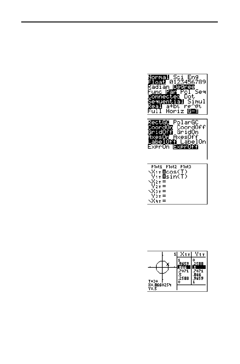
9-2 Split Screen
8309SPLT.DOC TI-83 international English Bob Fedorisko Revised: 02/19/01 12:31 PM Printed: 02/19/01 1:36
PM Page 2 of 6
Getting Started is a fast-paced introduction. Read the chapter for details.
Use
G
.
T (graph-table) split-screen mode to explore the unit circle and its
relationship to the numeric values for the commonly used trigonometric angles
of 0
°
, 30
°
, 45
°
, 60
°
, 90
°
, and so on.
1. Press
z
to display the mode screen.
Press
†
†
~
Í
to select
Degree
mode. Press
†
~
Í
to select Par
(parametric) graphing mode.
Press
†
†
†
†
~
~
Í
to select
G
.
T
(graph-table) split-screen mode.
2. Press
y
[
FORMAT
] to display the format
screen. Press
†
†
†
†
†
~
Í
to
select
ExprOff.
3. Press
o
to display the
Y=
editor for Par
graphing mode. Press
™
„
¤
Í
to store
cos(T) to X
1T
. Press
˜
„
¤
Í
to store
sin(T) to Y
1T
.
4. Press
p
to display the window
editor. Enter these values for the window
variables.
Tmin=0 Xmin=
L
2.3 Ymin=
L
2.5
Tmax=360 Xmax=2.3 Ymax=2.5
Tstep=15 Xscl=1 Yscl=1
5. Press
r
. On the left, the unit circle is
graphed parametrically in
Degree mode
and the trace cursor is activated. When
T=0 (from the graph trace coordinates),
you can see from the table on the right
that the value of
X
1T
(cos(T)) is 1 and Y
1T
(sin(T)) is 0. Press
~
to move the cursor to
the next 15
°
angle increment. As you trace
around the circle in steps of 15
°
, an
approximation of the standard value for
each angle is highlighted in the table.
Getting Started: Exploring the Unit Circle
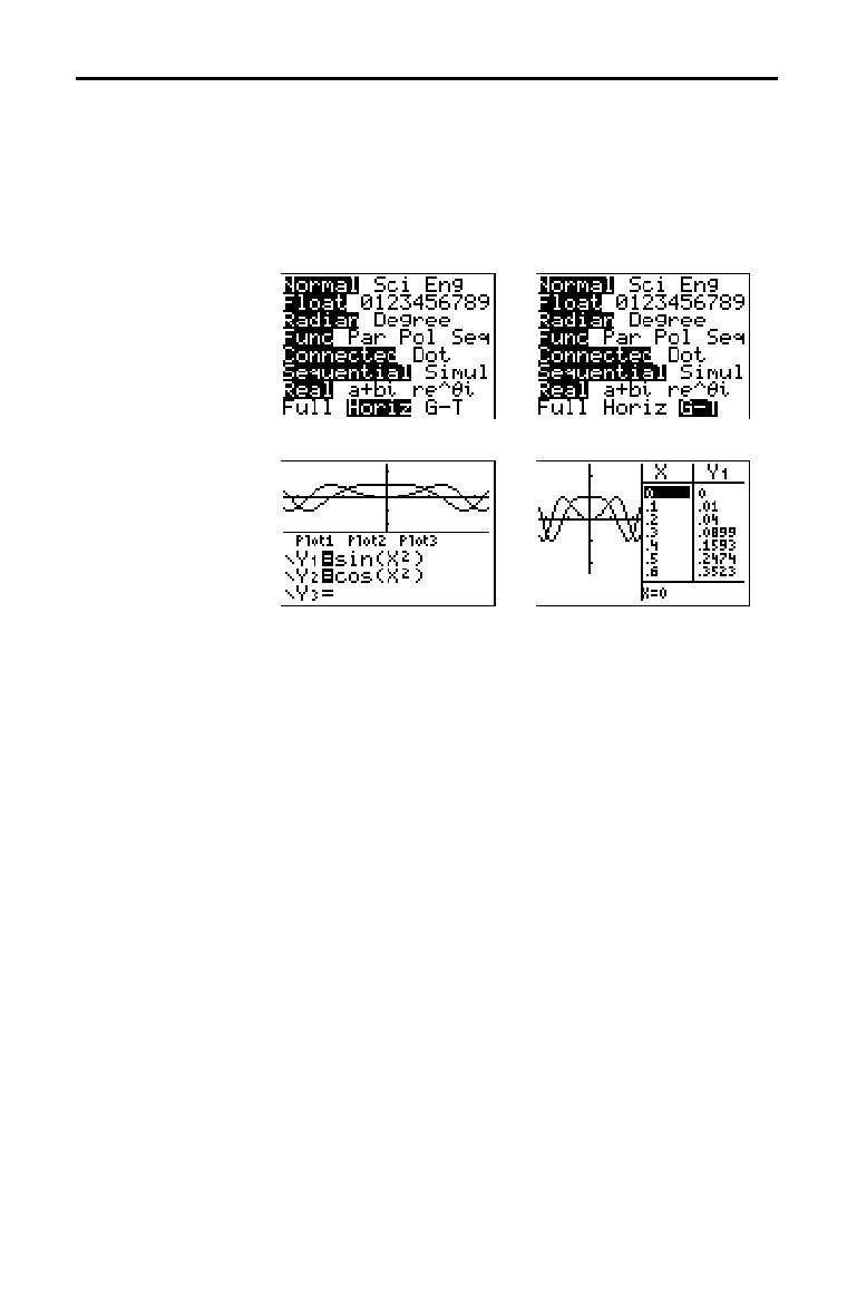
Split Screen 9-3
8309SPLT.DOC TI-83 international English Bob Fedorisko Revised: 02/19/01 12:31 PM Printed: 02/19/01 1:36
PM Page 3 of 6
To set a split-screen mode, press
z
, and then move the
cursor to the bottom line of the mode screen.
•
Select
Horiz (horizontal) to display the graph screen and
another screen split horizontally.
•
Select
G
.
T (graph-table) to display the graph screen and
table screen split vertically.
$$
The split screen is activated when you press any key that
applies to either half of the split screen.
Some screens are never displayed as split screens. For
example, if you press
z
in
Horiz or G
.
T mode, the mode
screen is displayed as a full screen. If you then press a key
that displays either half of a split screen, such as
r
,
the split screen returns.
When you press a key or key combination in either
Horiz or
G
.
T mode, the cursor is placed in the half of the display for
which that key applies. For example, if you press
r
,
the cursor is placed in the half in which the graph is
displayed. If you press
y
[
TABLE
], the cursor is placed in
the half in which the table is displayed.
The TI
-
83 will remain in split-screen mode until you
change back to
Full screen mode.
Using Split Screen
Setting a Split-
Screen Mode
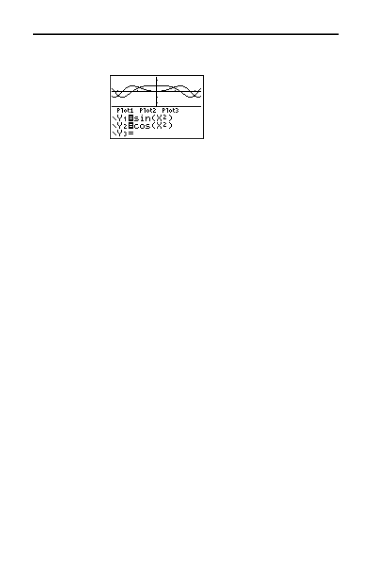
9-4 Split Screen
8309SPLT.DOC TI-83 international English Bob Fedorisko Revised: 02/19/01 12:31 PM Printed: 02/19/01 1:36
PM Page 4 of 6
In Horiz (horizontal) split-screen mode, a horizontal line
splits the screen into top and bottom halves.
The top half displays the graph.
The bottom half displays any of these editors.
•
Home screen (four lines)
•
Y=
editor (four lines)
•
Stat list editor (two rows)
•
Window editor (three settings)
•
Table editor (two rows)
To use the top half of the split screen:
•
Press
s
or
r
.
•
Select a
ZOOM
or
CALC
operation.
To use the bottom half of the split screen:
•
Press any key or key combination that displays the
home screen.
•
Press
o
(
Y=
editor).
•
Press
…
Í
(stat list editor).
•
Press
p
(window editor).
•
Press
y
[
TABLE
] (table editor).
All other screens are displayed as full screens in
Horiz
split-screen mode.
To return to the
Horiz split screen from a full screen when
in
Horiz mode, press any key or key combination that
displays the graph, home screen,
Y=
editor, stat list editor,
window editor, or table editor.
Horiz (Horizontal) Split Screen
Horiz Mode
Moving from Half
to Half in Horiz
Mode
Full Screens in
Horiz Mode
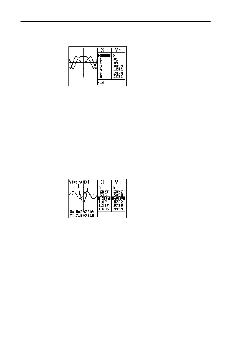
Split Screen 9-5
8309SPLT.DOC TI-83 international English Bob Fedorisko Revised: 02/19/01 12:31 PM Printed: 02/19/01 1:36
PM Page 5 of 6
In G
.
T (graph-table) split-screen mode, a vertical line splits
the screen into left and right halves.
The left half displays the graph.
The right half displays the table.
To use the left half of the split screen:
•
Press
s
or
r
.
•
Select a
ZOOM
or
CALC
operation.
To use the right half of the split screen, press
y
[
TABLE
].
As you move the trace cursor along a graph in the split
screen’s left half in
G
.
T mode, the table on the right half
automatically scrolls to match the current cursor values.
Note:
When you trace in
Par
graphing mode, both components of an
equation (
X
n
T
and
Y
n
T
) are displayed in the two columns of the table.
As you trace, the current value of the independent variable
T
is
displayed on the graph.
All screens other than the graph and the table are
displayed as full screens in
G
.
T split-screen mode.
To return to the
G
.
T split screen from a full screen when in
G
.
T mode, press any key or key combination that displays
the graph or the table.
G-T (Graph-Table) Split Screen
G-T Mode
Moving from Half
to Half in G-T
Mode
Using
r
in
G-T Mode
Full Screens in
G
.
T Mode
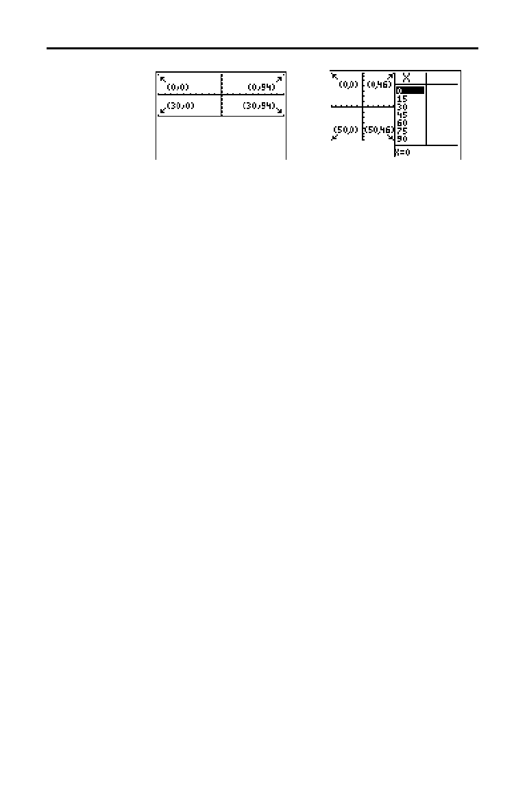
9-6 Split Screen
8309SPLT.DOC TI-83 international English Bob Fedorisko Revised: 02/19/01 12:31 PM Printed: 02/19/01 1:36
PM Page 6 of 6
Note:
Each set of numbers in parentheses above represents the row
and column of a corner pixel, which is turned on.
For
Pxl
.
On(
,
Pxl
.
Off(
,
Pxl
.
Change(
, and
pxl
.
Test(
:
•
In
Horiz
mode,
row
must be
{
30;
column
must be
{
94.
•
In
G
.
T
mode,
row
must be
{
50;
column
must be
{
46.
Pxl
.
On(
row
,
column
)
For the
Text(
instruction:
•
In
Horiz
mode,
row
must be
{
25;
column
must be
{
94.
•
In
G
.
T
mode,
row
must be
{
45;
column
must be
{
46.
Text(
row
,
column
,"
text
")
For the
Output(
instruction:
•
In
Horiz
mode,
row
must be
{
4;
column
must be
{
16.
•
In
G
.
T
mode,
row
must be
{
8;
column
must be
{
16.
Output(
row
,
column
,"
text
")
To set
Horiz
or
G
.
T
from a program, follow these steps.
1. Press
z
while the cursor is on a blank line in the
program editor.
2. Select
Horiz
or
G
.
T
.
The instruction is pasted to the cursor location. The mode
is set when the instruction is encountered during program
execution. It remains in effect after execution.
Note:
You also can paste
Horiz
or
G
.
T
to the home screen or
program editor from the
CATALOG
(Chapter 15).
TI-83 Pixels in Horiz and G-T Modes
TI-83 Pixels in
Horiz and G-T
Modes
DRAW POINTS
Menu Pixel
Instructions
DRAW Menu
Text( Instruction
PRGM I/O Menu
Output(
Instruction
Setting a
Split-Screen
Mode from the
Home Screen or
a Program
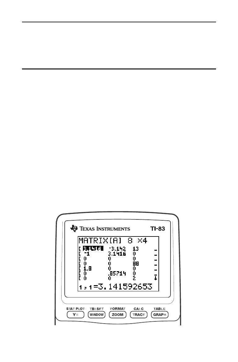
Matrices 10-1
8310MTRX.DOC TI-83 international English Bob Fedorisko Revised: 02/19/01 12:35 PM Printed: 02/19/01 1:36
PM Page 1 of 16
10
Matrices
Getting Started: Systems of Linear Equations
............
10-2
Defining a Matrix
........................................
10-2
Viewing and Editing Matrix Elements
....................
10-4
Using Matrices with Expressions
........................
10-7
Displaying and Copying Matrices
........................
10-8
Using Math Functions with Matrices
.....................
10-9
Using the
MATRX MATH
Operations
.....................
10-12
Contents
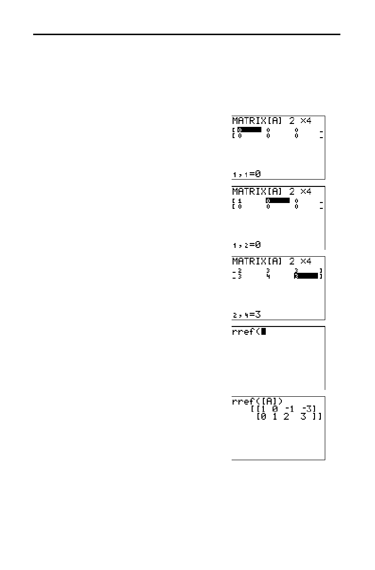
10-2 Matrices
8310MTRX.DOC TI-83 international English Bob Fedorisko Revised: 02/19/01 12:35 PM Printed: 02/19/01 1:36
PM Page 2 of 16
Getting Started is a fast-paced introduction. Read the chapter for details.
Find the solution of X + 2Y + 3Z = 3 and 2X + 3Y + 4Z = 3. On the TI
-
83, you
can solve a system of linear equations by entering the coefficients as elements
in a matrix, and then using
rref( to obtain the reduced row-echelon form.
1. Press
. Press
~
~
to display the
MATRX EDIT
menu. Press 1 to select 1: [A]¸
2. Press
2
Í
4
Í
to define a 2×4
matrix. The rectangular cursor indicates
the current element. Ellipses (
...) indicate
additional columns beyond the screen.
3. Press 1
Í
to enter the first element.
The rectangular cursor moves to the
second column of the first row.
4. Press 2
Í
3
Í
3
Í
to complete
the first row for X + 2Y + 3Z = 3.
5. Press
2
Í
3
Í
4
Í
3
Í
to
enter the second row for 2X + 3Y + 4Z = 3.
6. Press
y
[
QUIT
] to return to the home
screen. If necessary, press
‘
to clear
the home screen. Press
~
to
display the
MATRX MATH
menu. Press
}
to
wrap to the end of the menu. Select
B:rref(
to copy rref( to the home screen.
7. Press
1 to select 1: [A] from the
MATRX NAMES
menu. Press
¤
Í
. The
reduced row-echelon form of the matrix is
displayed and stored in
Ans.
1X
N
1Z =
L
3 so X =
L
3 + Z
1Y + 2Z = 3 so Y = 3
N
2Z
Getting Started: Systems of Linear Equations
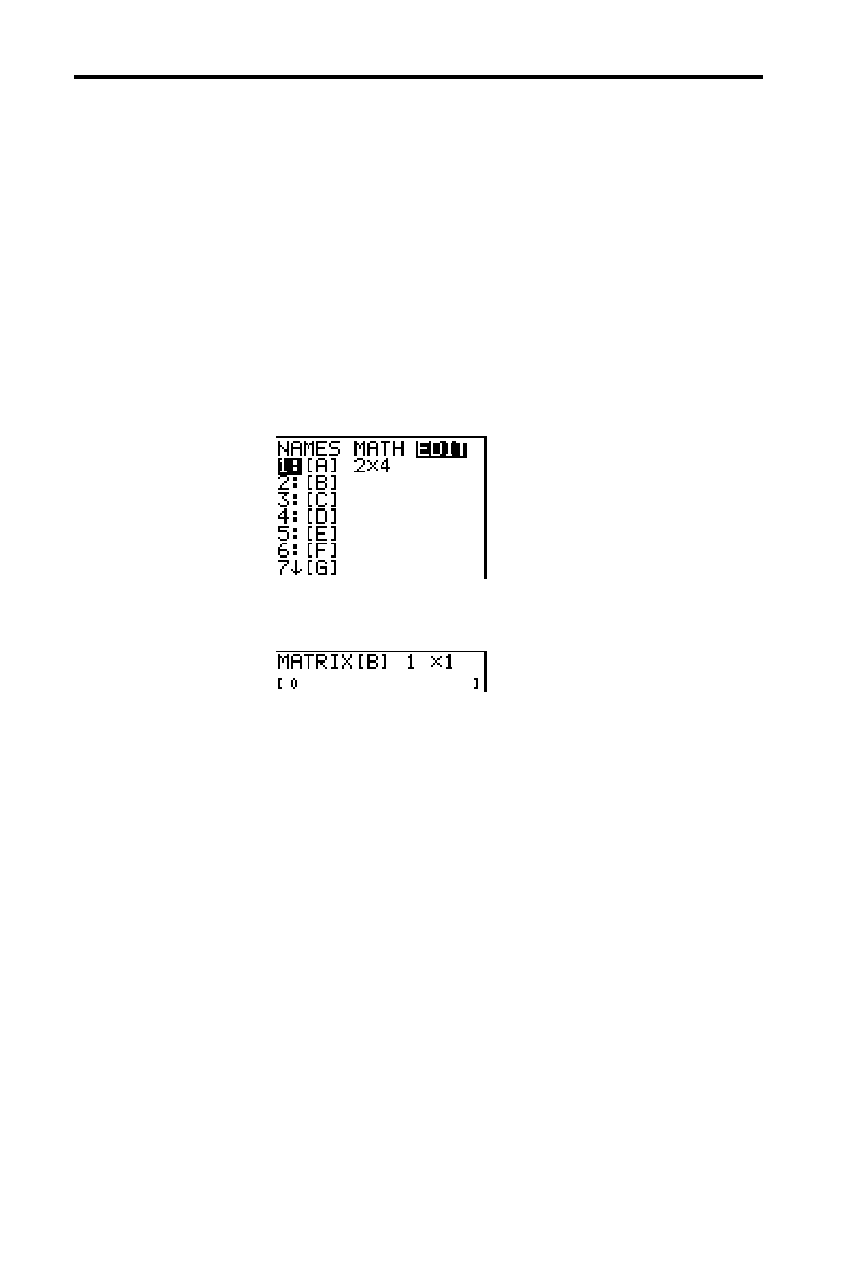
Matrices 10-3
8310MTRX.DOC TI-83 international English Bob Fedorisko Revised: 02/19/01 12:35 PM Printed: 02/19/01 1:36
PM Page 3 of 16
A matrix is a two-dimensional array. You can display,
define, or edit a matrix in the matrix editor. The TI
-
83 has
10 matrix variables,
[A] through [J]. You can define a
matrix directly in an expression. A matrix, depending on
available memory, may have up to 99 rows or columns.
You can store only real numbers in TI
-
83 matrices.
Before you can define or display a matrix in the editor, you
first must select the matrix name. To do so, follow these
steps.
1. Press
|
to display the
MATRX EDIT
menu. The
dimensions of any previously defined matrices are
displayed.
2. Select the matrix you want to define. The
MATRX EDIT
screen is displayed.
The dimensions of the matrix (
row
×
column
) are
displayed on the top line. The dimensions of a new matrix
are
1 ×1. You must accept or change the dimensions each
time you edit a matrix. When you select a matrix to define,
the cursor highlights the row dimension.
•
To accept the row dimension, press
Í
.
•
To change the row dimension, enter the number of rows
(up to
99), and then press
Í
.
The cursor moves to the column dimension, which you
must accept or change the same way you accepted or
changed the row dimension. When you press
Í
, the
rectangular cursor moves to the first matrix element.
Defining a Matrix
What Is a Matrix?
Selecting a
Matrix
Accepting or
Changing Matrix
Dimensions
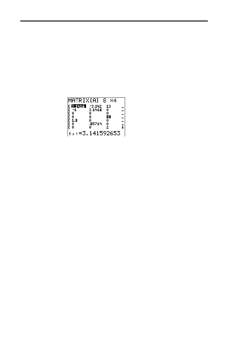
10-4 Matrices
8310MTRX.DOC TI-83 international English Bob Fedorisko Revised: 02/19/01 12:35 PM Printed: 02/19/01 1:36
PM Page 4 of 16
After you have set the dimensions of the matrix, you can
view the matrix and enter values for the matrix elements.
In a new matrix, all values are zero.
Select the matrix from the
MATRX EDIT
menu and enter or
accept the dimensions. The center portion of the matrix
editor displays up to seven rows and three columns of a
matrix, showing the values of the elements in abbreviated
form if necessary. The full value of the current element,
which is indicated by the rectangular cursor, is displayed
on the bottom line.
This is an 8 × 4 matrix. Ellipses in the left or right column
indicate additional columns.
#
or
$
in the right column
indicate additional rows.
To delete matrices from memory, use the
MEMORY DELETE
FROM
secondary menu (Chapter 18).
Viewing and Editing Matrix Elements
Displaying Matrix
Elements
Deleting a Matrix
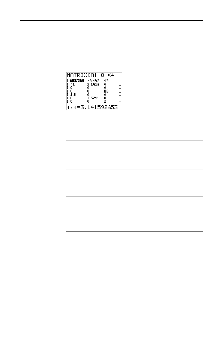
Matrices 10-5
8310MTRX.DOC TI-83 international English Bob Fedorisko Revised: 02/19/01 12:35 PM Printed: 02/19/01 1:36
PM Page 5 of 16
The matrix editor has two contexts, viewing and editing. In
viewing context, you can use the cursor keys to move
quickly from one matrix element to the next. The full value
of the highlighted element is displayed on the bottom line.
Select the matrix from the
MATRX EDIT
menu, and then
enter or accept the dimensions.
Key Function
|
or
~
Moves the rectan
g
ular cursor within the
current row.
†
or
}
Moves the rectan
g
ular cursor within the
current column; on the top row,
}
moves
the cursor to the column dimension; on the
column dimension,
}
moves the cursor to
the row dimension.
Í
Switches to editin
g
context; activates the
edit cursor on the bottom line.
‘
Switches to editin
g
context; clears the
v
alue on the bottom line.
A
ny entry
character
Switches to editin
g
context; clears the
v
alue on the bottom line; copies the
character to the bottom line.
y
[
INS
] Nothing
{
Nothing
Viewing a Matrix
Viewing-Context
Keys
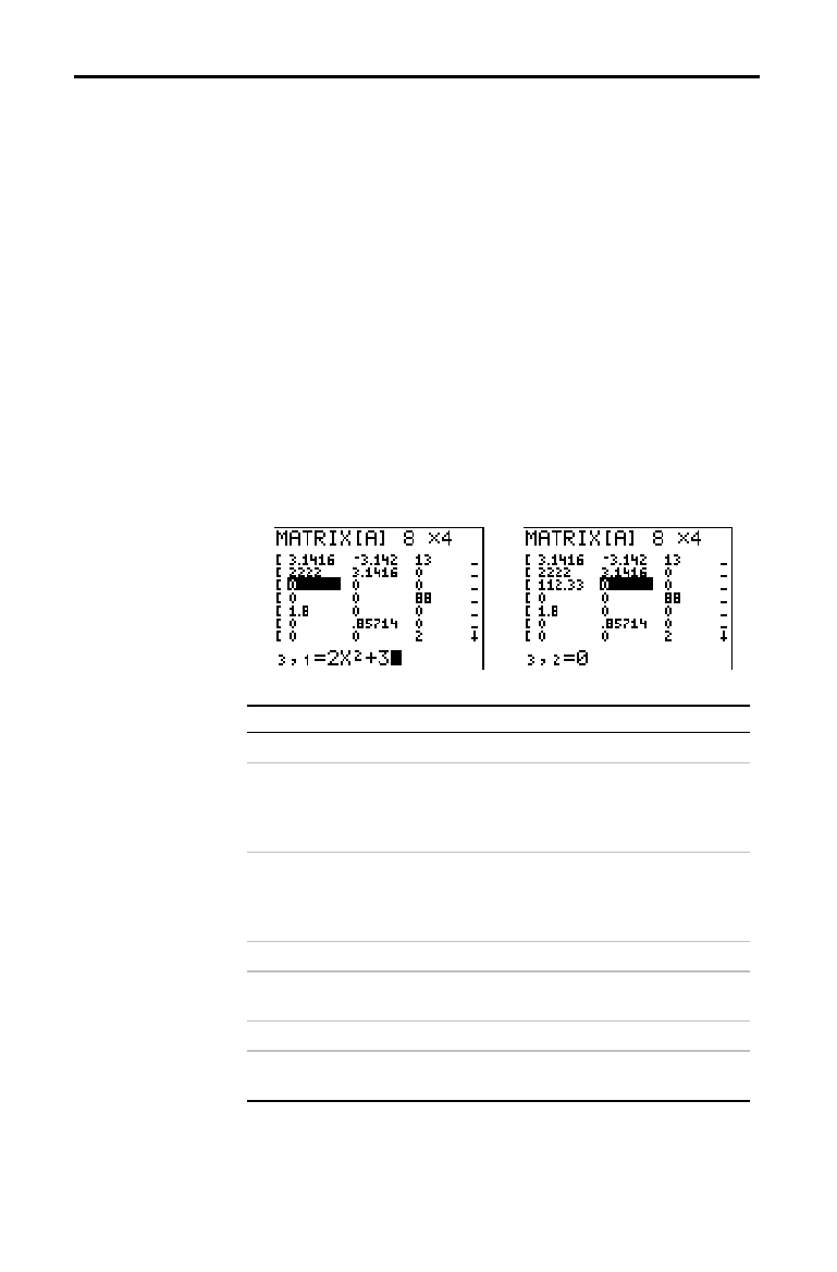
10-6 Matrices
8310MTRX.DOC TI-83 international English Bob Fedorisko Revised: 02/19/01 12:35 PM Printed: 02/19/01 1:36
PM Page 6 of 16
In editing context, an edit cursor is active on the bottom
line. To edit a matrix element value, follow these steps.
1. Select the matrix from the
MATRX EDIT
menu, and then
enter or accept the dimensions.
2. Press
|
,
}
,
~
, and
†
to move the cursor to the matrix
element you want to change.
3. Switch to editing context by pressing
Í
,
‘
, or
an entry key.
4. Change the value of the matrix element using the
editing-context keys described below. You may enter an
expression, which is evaluated when you leave editing
context.
Note:
You can press
‘
Í
to restore the value at the
rectangular cursor if you make a mistake.
5. Press
Í
,
}
, or
†
to move to another element.
Key Function
|
or
~
Moves the edit cursor within the value.
†
or
}
Stores the value displayed on the bottom
line to the matrix element; switches to
v
iewin
g
context and moves the rectan
g
ular
cursor within the column.
Í
Stores the value displayed on the bottom
line to the matrix element; switches to
v
iewin
g
context and moves the rectan
g
ular
cursor to the next row element.
‘
Clears the value on the bottom line.
A
ny entry
character
Copies the character to the location of the
edit cursor on the bottom line.
y
[
INS
] Activates the insert cursor.
{
Deletes the character under the edit cursor
on the bottom line.
Editing a Matrix
Element
Editing-Context
Keys
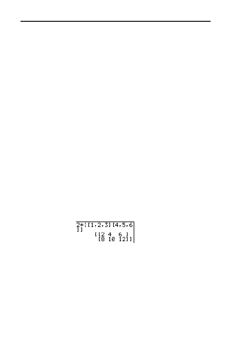
Matrices 10-7
8310MTRX.DOC TI-83 international English Bob Fedorisko Revised: 02/19/01 12:35 PM Printed: 02/19/01 1:36
PM Page 7 of 16
To use a matrix in an expression, you can do any of the
following.
•
Copy the name from the
MATRX NAMES
menu.
•
Recall the contents of the matrix into the expression
with
y
[
RCL
] (Chapter 1).
•
Enter the matrix directly (see below).
You can enter, edit, and store a matrix in the matrix editor.
You also can enter a matrix directly in an expression.
To enter a matrix in an expression, follow these steps.
1. Press
y
[
[ ] to indicate the beginning of the matrix.
2. Press
y
[
[ ] to indicate the beginning of a row.
3. Enter a value, which can be an expression, for each
element in the row. Separate the values with commas.
4. Press
y
[
] ] to indicate the end of a row.
5. Repeat steps 2 through 4 to enter all of the rows.
6. Press
y
[
] ] to indicate the end of the matrix.
Note:
The closing
]]
are not necessary at the end of an expression
or preceding
!
.
The resulting matrix is displayed in the form:
[[
element
1,1
,...,
element
1,n
],...,[
element
m,1
,...,
element
m,n
]]
Any expressions are evaluated when the entry is
executed.
Note:
The commas that you must enter to separate elements are
not displayed on output.
Using Matrices with Expressions
Using a Matrix in
an Expression
Entering a Matrix
in an Expression

10-8 Matrices
8310MTRX.DOC TI-83 international English Bob Fedorisko Revised: 02/19/01 12:35 PM Printed: 02/19/01 1:36
PM Page 8 of 16
To display the contents of a matrix on the home screen,
select the matrix from the
MATRX NAMES
menu, and then
press
Í
.
Ellipses in the left or right column indicate additional
columns.
#
or
$
in the right column indicate additional
rows. Press
~
,
|
,
†
, and
}
to scroll the matrix.
To copy a matrix, follow these steps.
1. Press
to display the
MATRX NAMES
menu.
2. Select the name of the matrix you want to copy.
3. Press
¿
.
4. Press
again and select the name of the new
matrix to which you want to copy the existing matrix.
5. Press
Í
to copy the matrix to the new matrix name.
On the home screen or from within a program, you can
store a value to, or recall a value from, a matrix element.
The element must be within the currently defined matrix
dimensions. Select
matrix
from the
MATRX NAMES
menu.
[
matrix
](
row
,
column
)
Displaying and Copying Matrices
Displaying a
Matrix
Copying One
Matrix to Another
Accessing a
Matrix Element
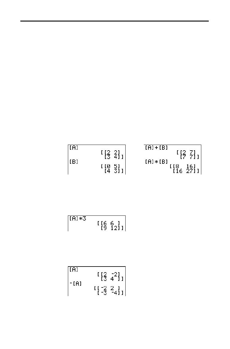
Matrices 10-9
8310MTRX.DOC TI-83 international English Bob Fedorisko Revised: 02/19/01 12:35 PM Printed: 02/19/01 1:36
PM Page 9 of 16
You can use many of the math functions on the TI
-
83
keyboard, the
MATH
menu, the
MATH NUM
menu, and the
MATH TEST
menu with matrices. However, the dimensions
must be appropriate. Each of the functions below creates a
new matrix; the original matrix remains the same.
To add (
Ã
) or subtract (
¹
) matrices, the dimensions must
be the same. The answer is a matrix in which the elements
are the sum or difference of the individual corresponding
elements.
matrixA
+
matrixB
matrixA
N
matrixB
To multiply (
¯
) two matrices together, the column
dimension of
matrixA
must match the row dimension of
matrixB
.
matrixA
ä
matrixB
Multiplying a
matrix
by a
value
or a
value
by a
matrix
returns a matrix in which each element of
matrix
is
multiplied by
value
.
matrix
ä
value
value
ä
matrix
Negating a matrix (
Ì
) returns a matrix in which the sign
of every element is changed (reversed).
L
matrix
Using Math Functions with Matrices
Using Math
Functions with
Matrices
+ (Add), –
(Subtract),
ä
(Multiply)
L
(Negation)
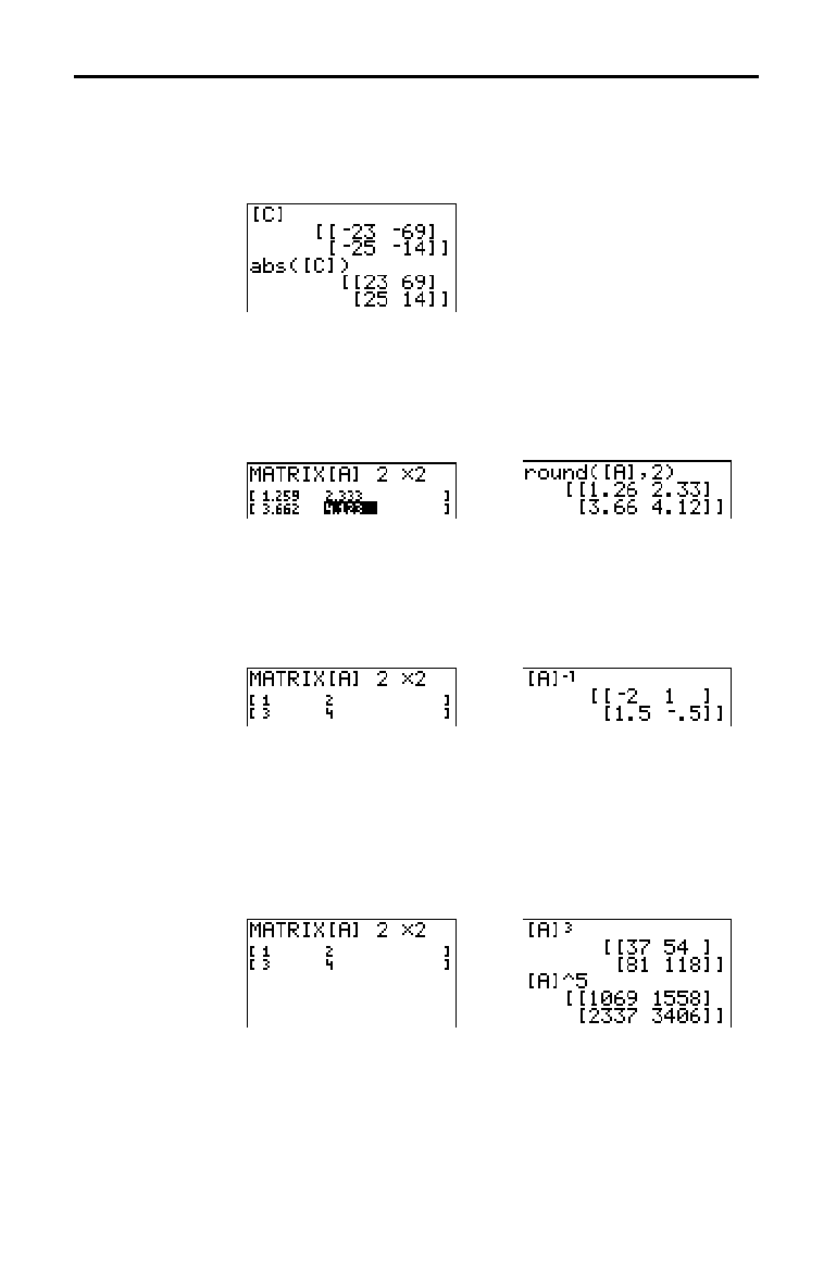
10-10 Matrices
8310MTRX.DOC TI-83 international English Bob Fedorisko Revised: 02/19/01 12:35 PM Printed: 02/19/01 1:36
PM Page 10 of 16
abs( (absolute value,
MATH NUM
menu) returns a matrix
containing the absolute value of each element of
matrix
.
abs(
matrix
)
round( (
MATH NUM
menu) returns a matrix. It rounds every
element in
matrix
to #
decimals
(
9). If
#decimals
is
omitted, the elements are rounded to 10 digits.
round(
matrix
[
,
#decimals
]
)
Use the
L
1
function (
—
) to invert a matrix (^
L
1 is not
valid).
matrix
must be square. The determinant cannot
equal zero.
matrix
L
1
To raise a matrix to a power,
matrix
must be square. You
can use
2
(
¡
),
3
(
MATH
menu), or ^
power
(
›
) for integer
power
between
0 and 255.
matrix
2
matrix
3
matrix
^
power
abs(
round(
M
1
(Inverse)
Powers
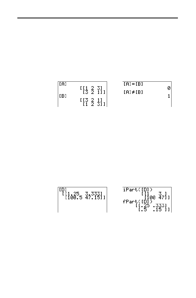
Matrices 10-11
8310MTRX.DOC TI-83 international English Bob Fedorisko Revised: 02/19/01 12:35 PM Printed: 02/19/01 1:36
PM Page 11 of 16
To compare two matrices using the relational operations =
and
ƒ
(
TEST
menu), they must have the same dimensions. =
and
ƒ
compare
matrixA
and
matrixB
on an element-by-
element basis. The other relational operations are not valid
with matrices.
matrixA
=
matrixB
returns
1 if every comparison is true; it
returns
0 if any comparison is false.
matrixA
ƒ
matrixB
returns
1 if at least one comparison is
false; it returns
0 if no comparison is false.
iPart( (integer part), fPart( (fractional part), and int(
(greatest integer) are on the
MATH NUM
menu.
iPart( returns a matrix containing the integer part of each
element of
matrix
.
fPart( returns a matrix containing the fractional part of
each element of
matrix
.
int( returns a matrix containing the greatest integer of each
element of
matrix
.
iPart(
matrix
)
fPart(
matrix
)
int(
matrix
)
Relational
Operations
iPart(, fPart(, int(
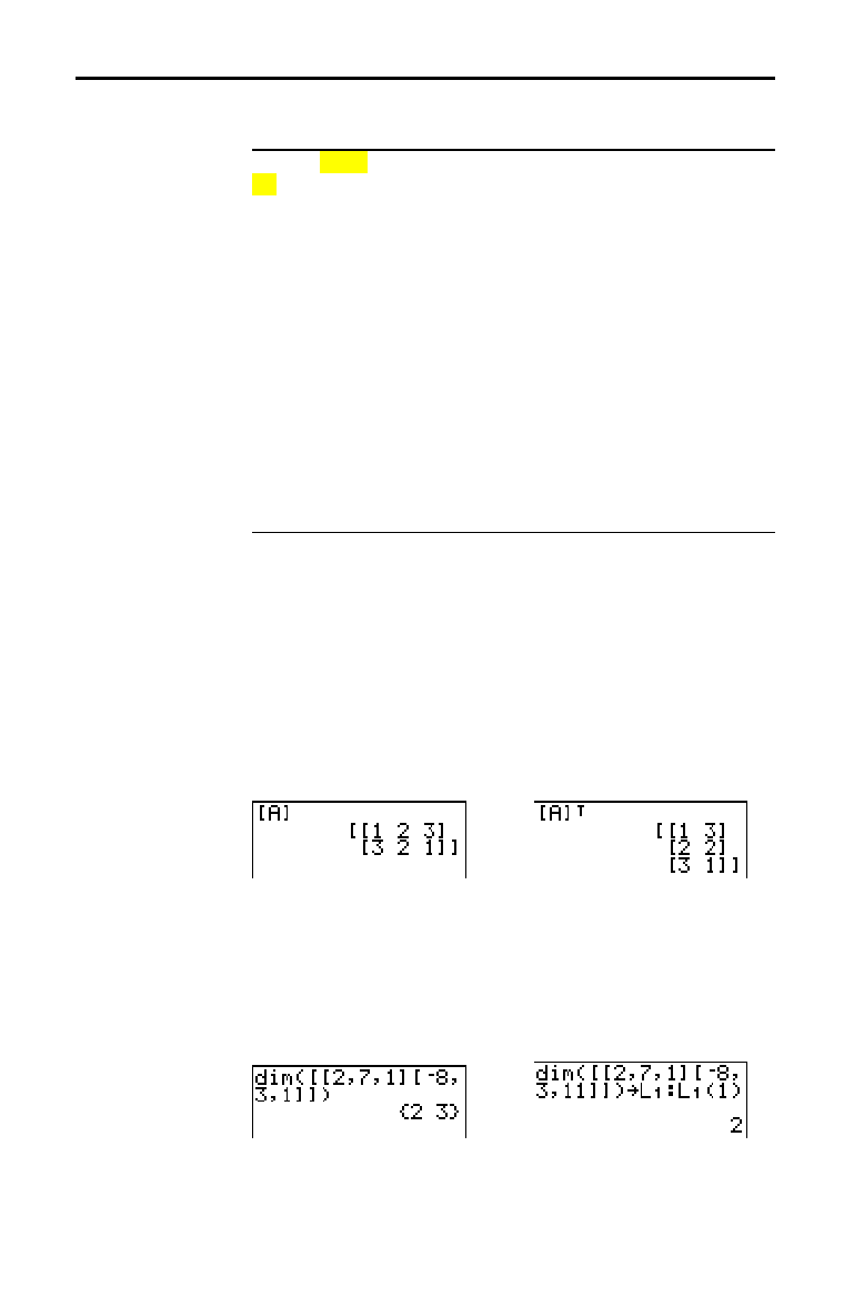
10-12 Matrices
8310MTRX.DOC TI-83 international English Bob Fedorisko Revised: 02/19/01 12:35 PM Printed: 02/19/01 1:36
PM Page 12 of 16
To display the
MATRX MATH
menu, press
~
.
NAMES MATH EDIT
1: det(
Calculates the determinant.
2:
T
Transposes the matrix.
3: dim(
Returns the matrix dimensions.
4: Fill(
Fills all elements with a constant.
5: identity(
Returns the identity matrix.
6: randM(
Returns a random matrix.
7: augment(
Appends two matrices.
8: Matr
4
list(
Stores a matrix to a list.
9: List
4
matr(
Stores a list to a matrix.
0: cumSum(
Returns the cumulative sums of a matrix.
A: ref(
Returns the row-echelon form of a matrix.
B: rref(
Returns the reduced row-echelon form.
C: rowSwap(
Swaps two rows of a matrix.
D: row+(
Adds two rows; stores in the second row.
E:
ä
row(
Multiplies the row by a number.
F:
ä
row+(
Multiplies the row, adds to the second row.
det( (determinant) returns the determinant (a real number)
of a square
matrix
.
det(
matrix
)
T
(transpose) returns a matrix in which each element (row,
column) is swapped with the corresponding element
(column, row) of
matrix
.
matrix
T
dim( (dimension) returns a list containing the dimensions
(
{
rows
columns
}) of
matrix
.
dim(
matrix
)
Note:
dim(
matrix
)
!
L
n
:L
n
(1)
returns the number of rows.
dim(
matrix
)
!
L
n
:L
n
(2)
returns the number of columns.
Using the MATRX MATH Operations
MATRX MATH
Menu
det(
T
(Transpose)
Accessing Matrix
Dimensions with
dim(
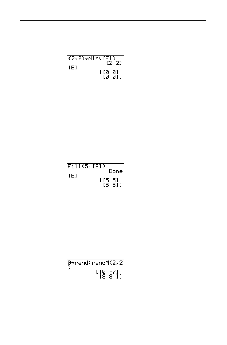
Matrices 10-13
8310MTRX.DOC TI-83 international English Bob Fedorisko Revised: 02/19/01 12:35 PM Printed: 02/19/01 1:36
PM Page 13 of 16
Use dim( with
¿
to create a new
matrixname
of
dimensions
rows
×
columns
with
0 as each element.
{
rows
,
columns
}
!
dim(
matrixname
)
Use dim( with
¿
to redimension an existing
matrixname
to dimensions
rows
×
columns
. The elements
in the old
matrixname
that are within the new dimensions
are not changed. Additional created elements are zeros.
Matrix elements that are outside the new dimensions are
deleted.
{
rows
,
columns
}
!
dim(
matrixname
)
Fill(
stores
value
to every element in
matrixname
.
Fill(
value
,
matrixname
)
identity( returns the identity matrix of
dimension
rows ×
dimension
columns.
identity(
dimension
)
randM(
(create random matrix) returns a
rows
×
columns
random matrix of integers
‚
L
9 and
9. The seed value
stored to the
rand function controls the values (Chapter 2).
randM(
rows
,
columns
)
Creating a Matrix
with dim(
Redimensioning a
Matrix with dim(
Fill(
identity(
randM(

10-14 Matrices
8310MTRX.DOC TI-83 international English Bob Fedorisko Revised: 02/19/01 12:35 PM Printed: 02/19/01 1:36
PM Page 14 of 16
augment( appends
matrixA
to
matrixB
as new columns.
matrixA
and
matrixB
both must have the same number of
rows.
augment(
matrixA
,
matrixB
)
Matr
4
list( (matrix stored to list) fills each
listname
with
elements from each column in
matrix
.
Matr
4
list( ignores
extra
listname
arguments. Likewise,
Matr
4
list( ignores
extra
matrix
columns.
Matr
4
list(
matrix
,
listnameA
,...,
listname n
)
&
Matr
4
list( also fills a
listname
with elements from a specified
column#
in
matrix
. To fill a list with a specific column from
matrix
, you must enter
column#
after
matrix
.
Matr
4
list(
matrix
,
column#
,
listname
)
&
List
4
matr( (lists stored to matrix) fills
matrixname
column by
column with the elements from each
list
. If dimensions of all
lists
are not equal,
List
4
matr( fills each extra
matrixname
row with
0. Complex lists are not valid.
List
4
matr(
listA
,...,
list n
,
matrixname
)
&
augment(
Matr
4
list(
List
4
matr(
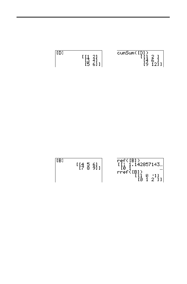
Matrices 10-15
8310MTRX.DOC TI-83 international English Bob Fedorisko Revised: 02/19/01 12:35 PM Printed: 02/19/01 1:36
PM Page 15 of 16
cumSum( returns cumulative sums of the elements in
matrix
, starting with the first element. Each element is the
cumulative sum of the column from top to bottom.
cumSum(
matrix
)
MATRX MATH
menu items A through F are row operations.
You can use a row operation in an expression. Row
operations do not change
matrix
in memory. You can
enter all row numbers and values as expressions. You can
select the matrix from the
MATRX NAMES
menu.
ref( (row-echelon form) returns the row-echelon form of a
real
matrix
. The number of columns must be greater than
or equal to the number of rows.
ref(
matrix
)
rref( (reduced row-echelon form) returns the reduced row-
echelon form of a real
matrix
. The number of columns must
be greater than or equal to the number of rows.
rref(
matrix
)
cumSum(
Row Operations
ref(, rref(
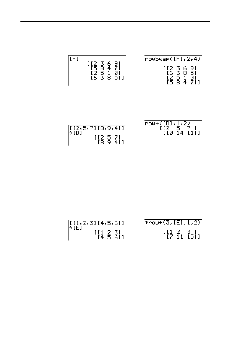
10-16 Matrices
8310MTRX.DOC TI-83 international English Bob Fedorisko Revised: 02/19/01 12:35 PM Printed: 02/19/01 1:36
PM Page 16 of 16
rowSwap( returns a matrix. It swaps
rowA
and
rowB
of
matrix
.
rowSwap(
matrix
,
rowA
,
rowB
)
row+( (row addition) returns a matrix. It adds
rowA
and
rowB
of
matrix
and stores the results in
rowB
.
row+(
matrix
,
rowA
,
rowB
)
ä
row(
(row multiplication) returns a matrix. It multiplies
row
of
matrix
by
value
and stores the results in
row
.
ä
row(
value
,
matrix
,
row
)
ä
row+(
(row multiplication and addition) returns a matrix.
It multiplies
rowA
of
matrix
by
value
, adds it to
rowB
, and
stores the results in
rowB
.
ä
row+(
value
,
matrix
,
rowA
,
rowB
)
rowSwap(
row+(
ä
row(
ä
row+(
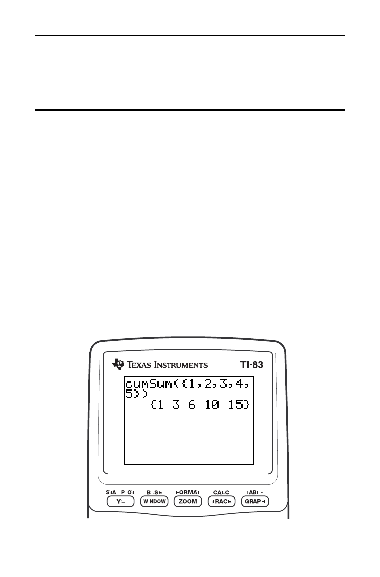
Lists 11-1
8311LIST.DOC TI-83 international English Bob Fedorisko Revised: 02/19/01 1:21 PM Printed: 02/19/01 1:37 PM
Page 1 of 18
11
Lists
Getting Started: Generating a Sequence
..................
11-2
Naming Lists
.............................................
11-3
Storing and Displaying Lists
.............................
11-4
Entering List Names
.....................................
11-6
Attaching Formulas to List Names
.......................
11-7
Using Lists in Expressions
...............................
11-9
LIST OPS
Menu
..........................................
11-10
LIST MATH
Menu
........................................
11-17
Contents
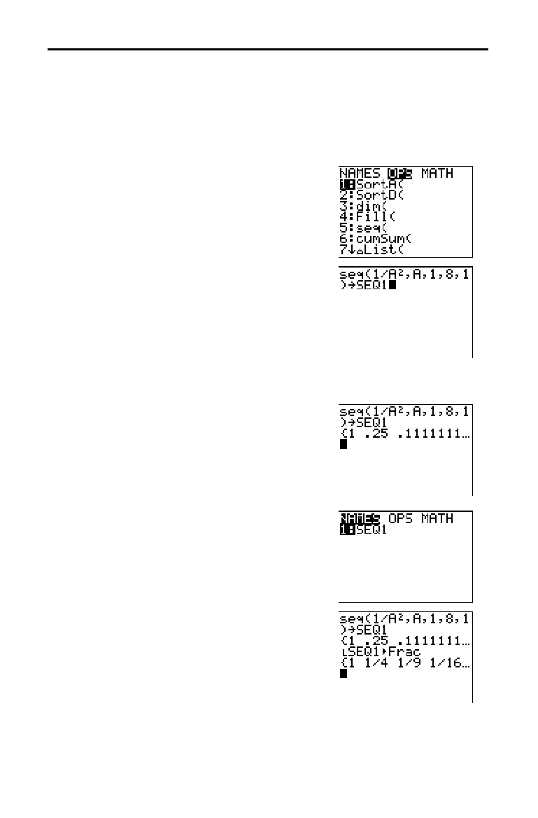
11-2 Lists
8311LIST.DOC TI-83 international English Bob Fedorisko Revised: 02/19/01 1:21 PM Printed: 02/19/01 1:37 PM
Page 2 of 18
Getting Started is a fast-paced introduction. Read the chapter for details.
Calculate the first eight terms of the sequence 1/A
2
. Store the results to a user-
created list. Then display the results in fraction form. Begin this example on a
blank line on the home screen.
1. Press
y
[
LIST
]
~
to display the
LIST OPS
menu.
2. Press 5 to select 5:seq(, which pastes seq( to
the current cursor location.
3. Press
1
¥
ƒ
[
A
]
¡
¢
ƒ
[
A
]
¢
1
¢
8
¢
1
¤
to enter the sequence.
4. Press
¿
, and then press
y
ƒ
to
turn on alpha-lock. Press [
S
] [
E
] [
Q
], and
then press
ƒ
to turn off alpha-lock.
Press
1 to complete the list name.
5. Press
Í
to generate the list and store it
in
SEQ1. The list is displayed on the home
screen. An ellipsis (
...) indicates that the list
continues beyond the viewing window.
Press
~
repeatedly (or press and hold
~
)
to scroll the list and view all the list
elements.
6. Press
y
[
LIST
] to display the
LIST NAMES
menu. Press
Í
to paste
Ù
SEQ1
to the
current cursor location. (If
SEQ1 is not item
1 on your
LIST NAMES
menu, move the
cursor to
SEQ1 before you press
Í
.)
7. Press
to display the
MATH
menu.
Press
1 to select 1:
4
Frac, which pastes
4
Frac
to the current cursor location.
8. Press
Í
to show the sequence in
fraction form. Press
~
repeatedly (or press
and hold
~
) to scroll the list and view all
the list elements.
Getting Started: Generating a Sequence
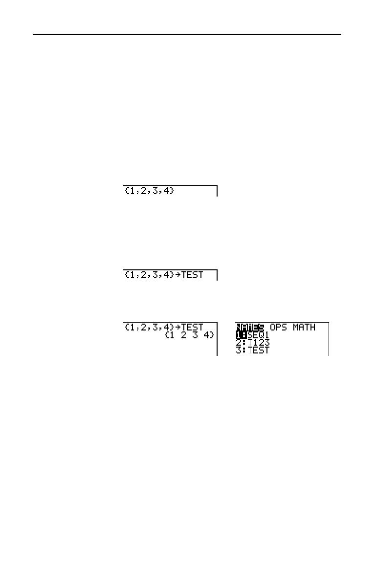
Lists 11-3
8311LIST.DOC TI-83 international English Bob Fedorisko Revised: 02/19/01 1:21 PM Printed: 02/19/01 1:37 PM
Page 3 of 18
The TI
-
83 has six list names in memory: L
1
, L
2
, L
3
, L
4
, L
5
,
and
L
6
. The list names L
1
through L
6
are on the keyboard
above the numeric keys
À
through
¸
. To paste one of
these names to a valid screen, press
y
, and then press
the appropriate key.
L
1
through L
6
are stored in stat list
editor columns
1 through 6 when you reset memory.
To create a list name on the home screen, follow these steps.
1. Press
y
[
{
], enter one or more list elements, and then
press
y
[
}
]. Separate list elements with commas. List
elements can be real numbers, complex numbers, or
expressions.
2. Press
¿
.
3. Press
ƒ
[
letter from A to Z or
q
] to enter the first
letter of the name.
4. Enter zero to four letters,
q
, or numbers to complete the
name.
5. Press
Í
. The list is displayed on the next line. The
list name and its elements are stored in memory. The
list name becomes an item on the
LIST NAMES
menu.
Note:
If you want to view a user-created list in the stat list editor,
you must store it in the stat list editor (Chapter 12).
You also can create a list name in these four places.
•
At the
Name= prompt in the stat list editor
•
At an
Xlist:, Ylist:, or Data List: prompt in the stat plot
editor
•
At a
List:, List1:, List2:, Freq:, Freq1:, Freq2:, XList:, or
YList: prompt in the inferential stat editors
•
On the home screen using
SetUpEditor
You can create as many list names as your TI
-
83 memory
has space to store.
Naming Lists
Using TI-83 List
Names L
1
through L
6
Creating a List
Name on the
Home Screen
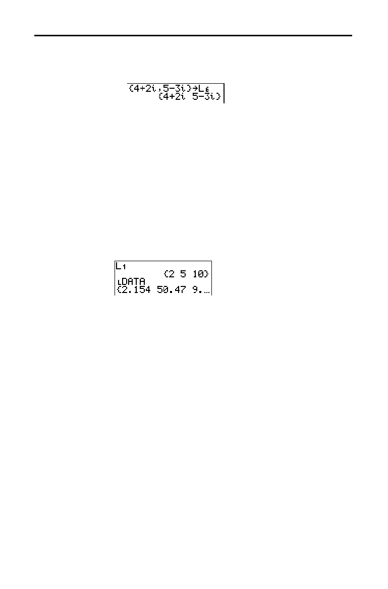
11-4 Lists
8311LIST.DOC TI-83 international English Bob Fedorisko Revised: 02/19/01 1:21 PM Printed: 02/19/01 1:37 PM
Page 4 of 18
You can store list elements in either of two ways.
•
Use braces and
¿
on the home screen.
•
Use the stat list editor (Chapter 12).
The maximum dimension of a list is 999 elements.
Tip:
When you store a complex number to a list, the entire list is
converted to a list of complex numbers. To convert the list to a list of
real numbers, display the home screen, and then enter
real(
listname
)
!
listname
.
To display the elements of a list on the home screen, enter
the name of the list (preceded by
Ù
if necessary; see page
11
.
16), and then press
Í
. An ellipsis indicates that the
list continues beyond the viewing window. Press
~
repeatedly (or press and hold
~
) to scroll the list and view
all the list elements.
Storing and Displaying Lists
Storing Elements
to a List
Displaying a List
on the Home
Screen
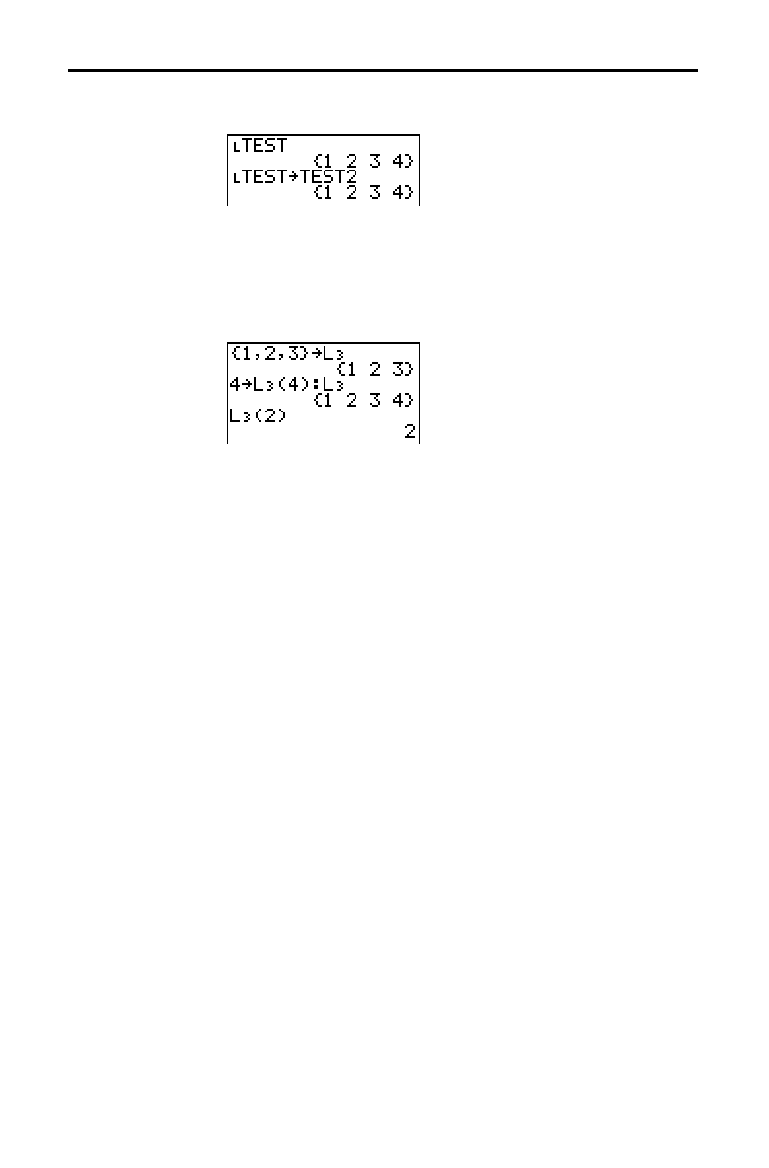
Lists 11-5
8311LIST.DOC TI-83 international English Bob Fedorisko Revised: 02/19/01 1:21 PM Printed: 02/19/01 1:37 PM
Page 5 of 18
To copy a list, store it to another list.
You can store a value to or recall a value from a specific
list
element
. You can store to any element within the
current list dimension or one element beyond.
listname
(
element
)
To delete lists from memory, including L
1
through L
6
, use the
MEMORY DELETE FROM
secondary menu (Chapter 18).
Resetting memory restores
L
1
through L
6
. Removing a list
from the stat list editor does not delete it from memory.
You can use lists to graph a family of curves (Chapter 3).
Copying One List
to Another
Accessing a List
Element
Deleting a List
from Memory
Using Lists in
Graphing
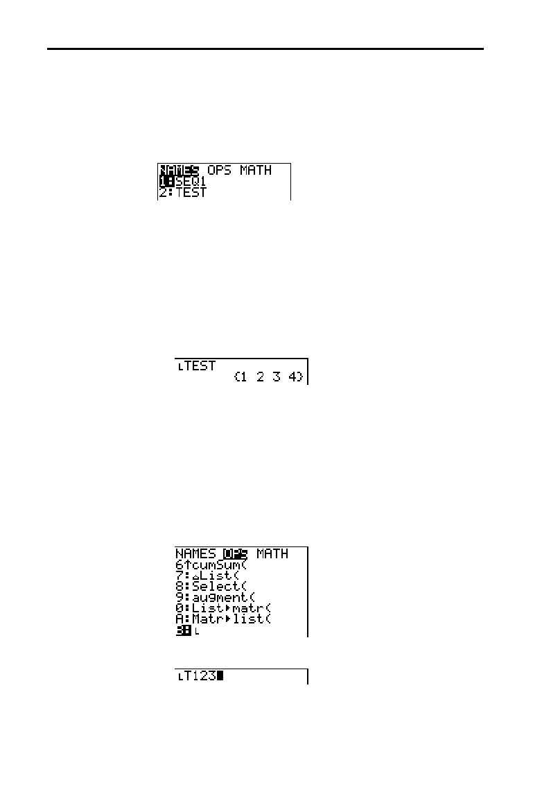
11-6 Lists
8311LIST.DOC TI-83 international English Bob Fedorisko Revised: 02/19/01 1:21 PM Printed: 02/19/01 1:37 PM
Page 6 of 18
To display the
LIST NAMES
menu, press
y
[
LIST
]. Each
item is a user-created list name.
LIST NAMES
menu items are
sorted automatically in alphanumerical order. Only the first
10 items are labeled, using
1 through 9, then 0. To jump to
the first list name that begins with a particular alpha
character or
q
, press
ƒ
[
letter from A to Z or
q
].
Tip:
From the top of a menu, press
}
to move to the bottom. From the
bottom, press
†
to move to the top.
Note:
The
LIST NAMES
menu omits list names
L
1
through
L
6
. Enter
L1
through
L
6
directly from the keyboard (page 11
.
3).
When you select a list name from the
LIST NAMES
menu,
the list name is pasted to the current cursor location.
•
The list name symbol
Ù
precedes a list name when the
name is pasted where non-list name data also is valid,
such as the home screen.
•
The
Ù
symbol does not precede a list name when the
name is pasted where a list name is the only valid input,
such as the stat list editor’s Name= prompt or the stat
plot editor’s XList: and YList: prompts.
To enter an existing list name directly, follow these steps.
1. Press
y
[
LIST
]
~
to display the
LIST OPS
menu.
2. Select
B:
Ù
, which pastes
Ù
to the current cursor location.
Ù
is not always necessary (page 11
.
16).
Note:
You also can paste
Ù
to the
current cursor location from the
CATALOG
(Chapter 15).
3. Enter the characters that comprise the list name.
Entering List Names
Using the
LIST NAMES
Menu
Entering a User-
Created List
Name Directly
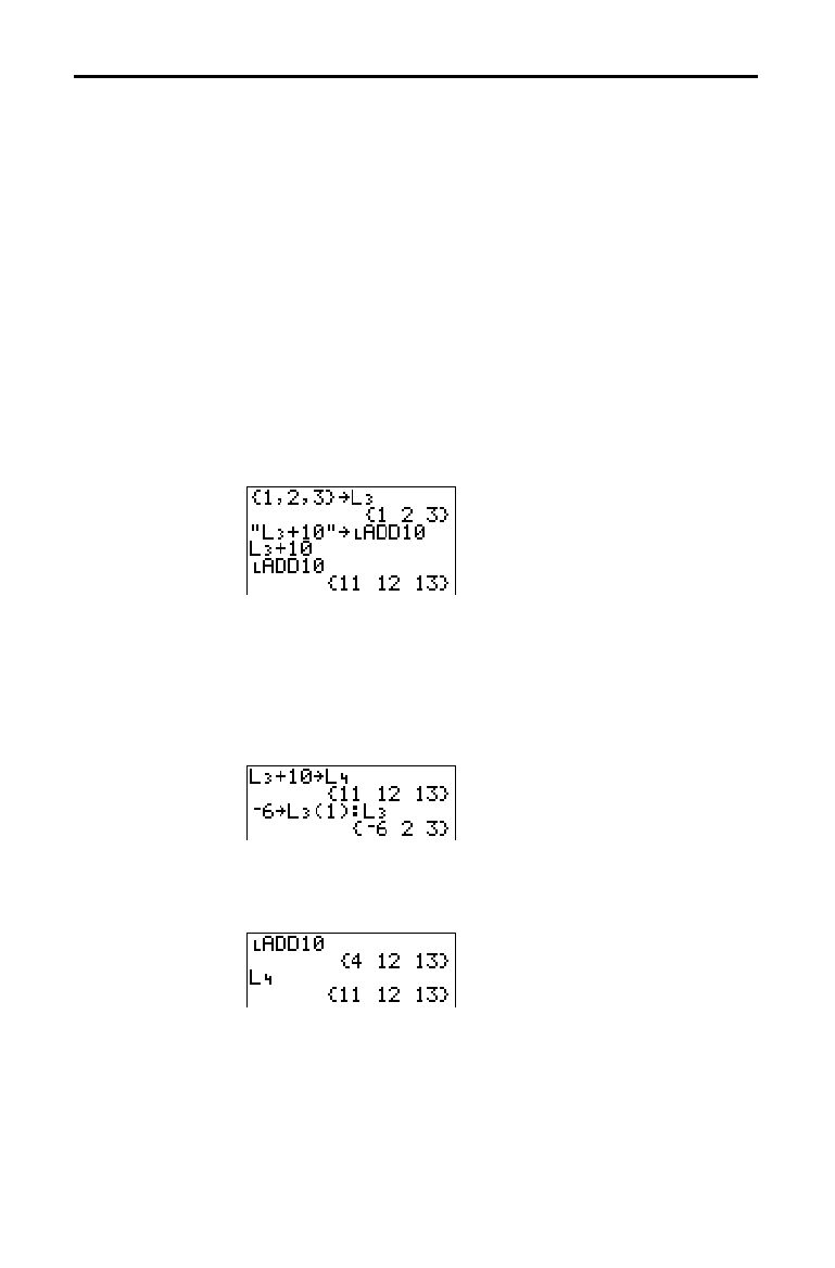
Lists 11-7
8311LIST.DOC TI-83 international English Bob Fedorisko Revised: 02/19/01 1:21 PM Printed: 02/19/01 1:37 PM
Page 7 of 18
You can attach a formula to a list name so that each list
element is a result of the formula. When executed, the
attached formula must resolve to a list.
When anything in the attached formula changes, the list to
which the formula is attached is updated automatically.
•
When you edit an element of a list that is referenced in
the formula, the corresponding element in the list to
which the formula is attached is updated.
•
When you edit the formula itself, all elements in the list
to which the formula is attached are updated.
For example, the first screen below shows that elements
are stored to
L
3
, and the formula L
3
+10 is attached to the
list name
Ù
ADD10
. The quotation marks designate the
formula to be attached to
Ù
ADD10
. Each element of
Ù
ADD10
is the sum of an element in L
3
and 10.
The next screen shows another list, L
4
. The elements of L
4
are the sum of the same formula that is attached to L
3
.
However, quotation marks are not entered, so the formula
is not attached to
L
4
.
On the next line,
L
6
!
L
3
(1):L
3
changes the first element in L
3
to
L
6
, and then redisplays L
3
.
The last screen shows that editing L
3
updated
Ù
ADD10
, but
did not change
L
4
. This is because the formula L
3
+10 is
attached to
Ù
ADD10
, but it is not attached to L
4
.
Note:
To view a formula that is attached to a list name, use the stat list
editor (Chapter 12).
Attaching Formulas to List Names
Attaching a
Formula to a List
Name
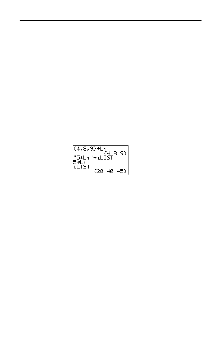
11-8 Lists
8311LIST.DOC TI-83 international English Bob Fedorisko Revised: 02/19/01 1:21 PM Printed: 02/19/01 1:37 PM
Page 8 of 18
To attach a formula to a list name from a blank line on the
home screen or from a program, follow these steps.
1. Press
ƒ
[
ã
], enter the formula (which must resolve to
a list), and press
ƒ
[
ã
] again.
Note:
When you include more than one list name in a formula,
each list must have the same dimension.
2. Press
¿
.
3. Enter the name of the list to which you want to attach
the formula.
•
Press
y
, and then enter a TI
-
83 list name
L
1
through
L
6
.
•
Press
y
[
LIST
] and select a user
.
created list name
from the
LIST NAMES
menu.
•
Enter a user
.
created list name directly using
Ù
(page
11
.
16).
4. Press
Í
.
Note:
The stat list editor displays a formula-lock symbol next to
each list name that has an attached formula. Chapter 12 describes
how to use the stat list editor to attach formulas to lists, edit
attached formulas, and detach formulas from lists.
You can detach (clear) an attached formula from a list in
any of three ways.
•
Enter
""
!
listname
on the home screen.
•
Edit any element of a list to which a formula is
attached.
•
Use the stat list editor (Chapter 12).
Note:
You also can use
ClrList
or
ClrAllList
to detach a formula
from a list (Chapter 18).
Attaching a
Formula to a List
on the Home
Screen or in a
Program
Detaching a
Formula from a
List
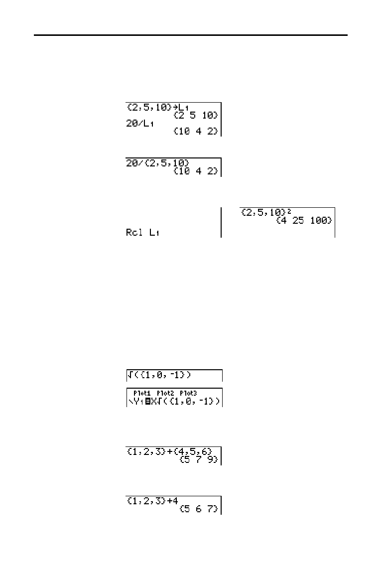
Lists 11-9
8311LIST.DOC TI-83 international English Bob Fedorisko Revised: 02/19/01 1:21 PM Printed: 02/19/01 1:37 PM
Page 9 of 18
You can use lists in an expression in any of three ways.
When you press
Í
, any expression is evaluated for
each list element, and a list is displayed.
•
Use
L
1
–L
6
or any user-created list name in an expression.
•
Enter the list elements directly (step 1 on page 11
.
3).
•
Use
y
[
RCL
] to recall the contents of the list into an
expression at the cursor location (Chapter 1).
&
Note:
You must paste user-created list names to the
Rcl
prompt by
selecting them from the
LIST NAMES
menu. You cannot enter them
directly using
Ù
.
You can use a list to input several values for some math
functions. Other chapters and Appendix A specify whether
a list is valid. The function is evaluated for each list
element, and a list is displayed.
•
When you use a list with a function, the function must
be valid for every element in the list. In graphing, an
invalid element, such as
L
1
in
‡
({1,0,
L
1})
, is ignored.
This returns an error.
This graphs
X
ä
‡
(1)
and
X
ä
‡
(0)
,
but skips
X
ä
‡
(
L
1)
.
•
When you use two lists with a two-argument function,
the dimension of each list must be the same. The
function is evaluated for corresponding elements.
•
When you use a list and a value with a two-argument
function, the value is used with each element in the list.
Using Lists in Expressions
Using a List in an
Expression
Using Lists with
Math Functions

11-10 Lists
8311LIST.DOC TI-83 international English Bob Fedorisko Revised: 02/19/01 1:21 PM Printed: 02/19/01 1:37 PM
Page 10 of 18
To display the
LIST OPS
menu, press
y
[
LIST
]
~
.
NAMES OPS MATH
1:SortA(
Sorts lists in ascending order.
2:SortD(
Sorts lists in descending order.
3:dim(
Sets the list dimension.
4:Fill(
Fills all elements with a constant.
5:seq(
Creates a sequence.
6:cumSum(
Returns a list of cumulative sums.
7:@List(
Returns difference of successive elements.
8:Select(
Selects specific data points.
9:augment(
Concatenates two lists.
0:List
4
matr(
Stores a list to a matrix.
A:Matr
4
list(
Stores a matrix to a list.
B:
Ù
Designates the list-name data type.
SortA( (sort ascending) sorts list elements from low to high
values.
SortD( (sort descending) sorts list elements from
high to low values. Complex lists are sorted based on
magnitude (modulus).
With one list,
SortA( and SortD( sort the elements of
listname
and update the list in memory.
SortA(
listname
) SortD(
listname
)
With two or more lists, SortA( and SortD( sort
keylistname
,
and then sort each
dependlist
by placing its elements in the
same order as the corresponding elements in
keylistname
.
All lists must have the same dimension.
SortA(
keylistname
,
dependlist1
[
,
dependlist2
,...,
dependlist n
]
)
SortD(
keylistname
,
dependlist1
[
,
dependlist2
,...,
dependlist n
]
)
Note:
In the example,
5
is the first element in
L
4
, and
1
is the first
element in
L
5
. After
SortA(L
4
,L
5
)
,
5
becomes the second element of
L
4
, and likewise,
1
becomes the second element of
L
5
.
Note:
SortA(
and
SortD(
are the same as
SortA(
and
SortD(
on the
STAT EDIT
menu (Chapter 12).
LIST OPS Menu
LIST OPS Menu
SortA(, SortD(
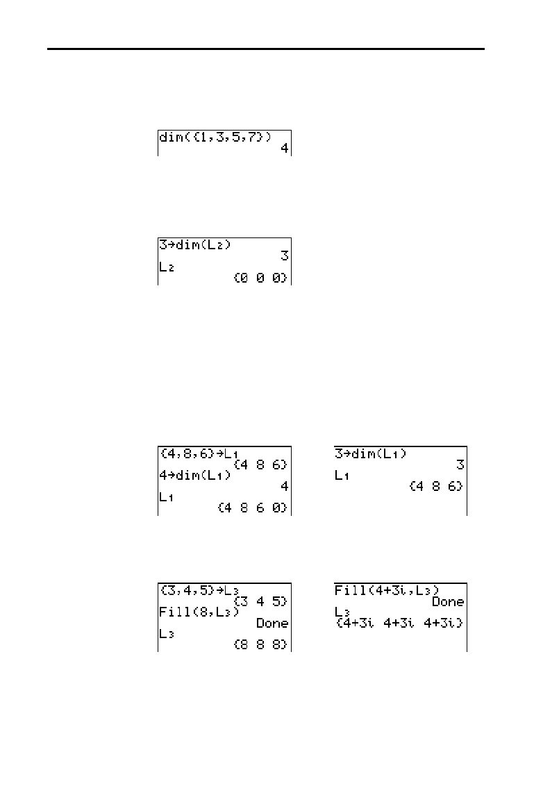
Lists 11-11
8311LIST.DOC TI-83 international English Bob Fedorisko Revised: 02/19/01 1:21 PM Printed: 02/19/01 1:37 PM
Page 11 of 18
dim( (dimension) returns the length (number of elements)
of
list
.
dim(
list
)
You can use dim( with
¿
to create a new
listname
with
dimension
length
from 1 to 999. The elements are zeros.
length
!
dim(
listname
)
You can use dim with
¿
to redimension an existing
listname
to dimension
length
from 1 to 999.
•
The elements in the old
listname
that are within the
new dimension are not changed.
•
Extra list elements are filled by
0.
•
Elements in the old list that are outside the new
dimension are deleted.
length
!
dim(
listname
)
Fill( replaces each element in
listname
with
value
.
Fill(
value
,
listname
)
Note:
dim(
and
Fill(
are the same as
dim(
and
Fill(
on the
MATRX
MATH
menu (Chapter 10).
Using dim( to
Find List
Dimensions
Using dim( to
Create a List
Using dim( to
Redimension a
List
Fill(
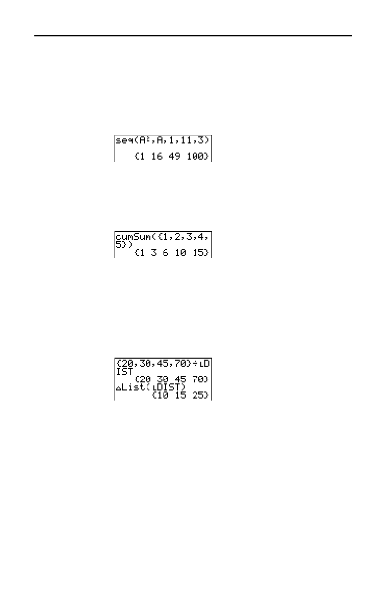
11-12 Lists
8311LIST.DOC TI-83 international English Bob Fedorisko Revised: 02/19/01 1:21 PM Printed: 02/19/01 1:37 PM
Page 12 of 18
seq( (sequence) returns a list in which each element is the
result of the evaluation of
expression
with regard to
variable
for the values ranging from
begin
to
end
at steps
of
increment
.
variable
need not be defined in memory.
increment
can be negative; the default value for
increment
is 1.
seq( is not valid within
expression
.
seq(
expression
,
variable
,
begin
,
end
[
,
increment
]
)
cumSum( (cumulative sum) returns the cumulative sums of
the elements in
list
, starting with the first element.
list
elements can be real or complex numbers.
cumSum(
list
)
@
List(
returns a list containing the differences between
consecutive elements in
list
.
@
List
subtracts the first
element in
list
from the second element, subtracts the
second element from the third, and so on. The list of
differences is always one element shorter than the original
list
.
list
elements can be a real or complex numbers.
@
List(
list
)
Select( selects one or more specific data points from a
scatter plot or xyLine plot (only), and then stores the
selected data points to two new lists,
xlistname
and
ylistname
. For example, you can use
Select( to select and
then analyze a portion of plotted CBL 2/CBL or CBR data.
Select(
xlistname
,
ylistname
)
Note:
Before you use
Select(
, you must have selected (turned on) a
scatter plot or xyLine plot. Also, the plot must be displayed in the
current viewing window (page 11
.
13).
seq(
cumSum(
@
List(
Select(
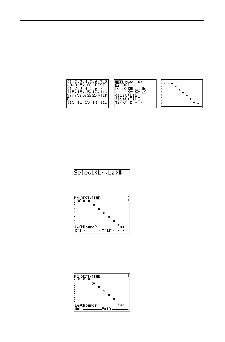
Lists 11-13
8311LIST.DOC TI-83 international English Bob Fedorisko Revised: 02/19/01 1:21 PM Printed: 02/19/01 1:37 PM
Page 13 of 18
Before using Select(, follow these steps.
1. Create two list names and enter the data.
2. Turn on a stat plot, select
"
(scatter plot) or
Ó
(xyLine),
and enter the two list names for
Xlist: and Ylist: (Chapter
12).
3. Use
ZoomStat to plot the data (Chapter 3).
To select data points from a scatter plot or xyLine plot,
follow these steps.
1. Press
y
[
LIST
]
~
8 to select 8:Select( from the
LIST
OPS
menu. Select( is pasted to the home screen.
2. Enter
xlistname
, press
¢
, enter
ylistname
, and then
press
¤
to designate list names into which you want
the selected data to be stored.
3. Press
Í
. The graph screen is displayed with
Left Bound? in the bottom-left corner.
4. Press
}
or
†
(if more than one stat plot is selected) to
move the cursor onto the stat plot from which you want
to select data points.
5. Press
|
and
~
to move the cursor to the stat plot data
point that you want as the left bound.
Before Using
Select(
Using Select( to
Select Data
Points from a
Plot
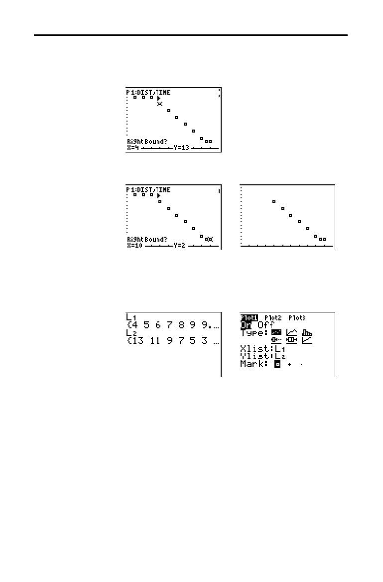
11-14 Lists
8311LIST.DOC TI-83 international English Bob Fedorisko Revised: 02/19/01 1:21 PM Printed: 02/19/01 1:37 PM
Page 14 of 18
6. Press
Í
. A
4
indicator on the graph screen shows
the left bound.
Right Bound? is displayed in the bottom-
left corner.
7. Press
|
or
~
to move the cursor to the stat plot point
that you want for the right bound, and then press
Í
.
The x-values and y-values of the selected points are
stored in
xlistname
and
ylistname
. A new stat plot of
xlistname
and
ylistname
replaces the stat plot from
which you selected data points. The list names are
updated in the stat plot editor.
Note:
The two new lists (
xlistname
and
ylistname
) will include the
points you select as left bound and right bound. Also,
left-bound
x-value
right-bound x-value
must be true.
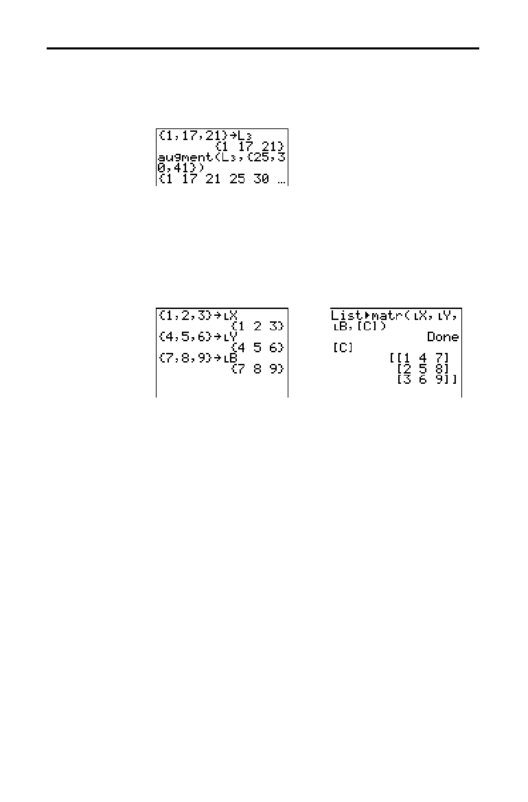
Lists 11-15
8311LIST.DOC TI-83 international English Bob Fedorisko Revised: 02/19/01 1:21 PM Printed: 02/19/01 1:37 PM
Page 15 of 18
augment( concatenates the elements of
listA
and
listB
. The
list elements can be real or complex numbers.
augment(
listA
,
listB
)
List
4
matr( (lists stored to matrix) fills
matrixname
column
by column with the elements from each list. If the
dimensions of all lists are not equal, then
List
4
matr( fills
each extra
matrixname
row with
0. Complex lists are not
valid.
List
4
matr(
list1
,
list2
, . . . ,
list n
,
matrixname
)
&
augment(
List
4
matr(
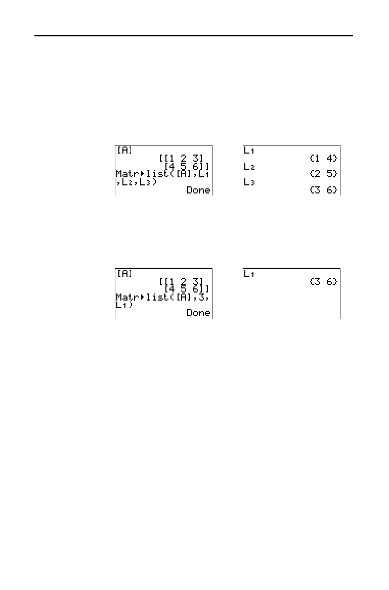
11-16 Lists
8311LIST.DOC TI-83 international English Bob Fedorisko Revised: 02/19/01 1:21 PM Printed: 02/19/01 1:37 PM
Page 16 of 18
Matr
4
list( (matrix stored to lists) fills each
listname
with
elements from each column in
matrix
. If the number of
listname
arguments exceeds the number of columns in
matrix
, then
Matr
4
list( ignores extra
listname
arguments.
Likewise, if the number of columns in
matrix
exceeds the
number of
listname
arguments, then
Matr
4
list( ignores
extra
matrix
columns.
Matr
4
list(
matrix
,
listname1
,
listname2
, . . . ,
listname n
)
&
Matr
4
list( also fills a
listname
with elements from a
specified
column#
in
matrix
. To fill a list with a specific
column from
matrix
, you must enter a
column#
after
matrix
.
Matr
4
list(
matrix
,
column#
,
listname
)
&
Ù
preceding one to five characters identifies those
characters as a user-created
listname
.
listname
may
comprise letters,
q
, and numbers, but it must begin with a
letter from A to Z or
q
.
Ù
listname
Generally,
Ù
must precede a user-created list name when
you enter a user-created list name where other input is
valid, for example, on the home screen. Without the
Ù
, the
TI
-
83 may misinterpret a user-created list name as implied
multiplication of two or more characters.
Ù
need not precede a user-created list name where a list
name is the only valid input, for example, at the
Name=
prompt in the stat list editor or the Xlist: and Ylist: prompts
in the stat plot editor. If you enter
Ù
where it is not
necessary, the TI
-
83 will ignore the entry.
Matr
4
list(

Lists 11-17
8311LIST.DOC TI-83 international English Bob Fedorisko Revised: 02/19/01 1:21 PM Printed: 02/19/01 1:37 PM
Page 17 of 18
To display the
LIST MATH
menu, press
y
[
LIST
]
|
.
NAMES OPS MATH
1: min(
Returns minimum element of a list.
2: max(
Returns maximum element of a list.
3: mean(
Returns mean of a list.
4: median(
Returns median of a list.
5: sum(
Returns sum of elements in a list.
6: prod(
Returns product of elements in list.
7: stdDev(
Returns standard deviation of a list.
8: variance(
Returns the variance of a list.
min( (minimum) and max( (maximum) return the smallest or
largest element of
listA
. If two lists are compared, it returns
a list of the smaller or larger of each pair of elements in
listA
and
listB
. For a complex list, the element with smallest or
largest magnitude (modulus) is returned.
min(
listA
[
,
listB
]
)
max(
listA
[
,
listB
]
)
Note:
min(
and
max(
are the same as
min(
and
max(
on the
MATH
NUM
menu.
mean( returns the mean value of
list
. median( returns the
median value of
list
. The default value for
freqlist
is 1.
Each
freqlist
element counts the number of consecutive
occurrences of the corresponding element in
list
. Complex
lists are not valid.
mean(
list
[
,
freqlist
]
)
median(
list
[
,
freqlist
]
)
LIST MATH Menu
LIST MATH Menu
min(, max(
mean(, median(
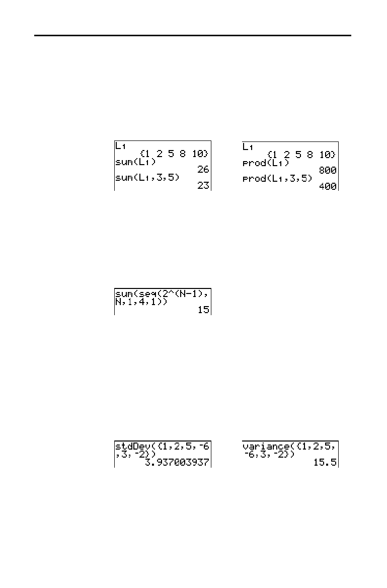
11-18 Lists
8311LIST.DOC TI-83 international English Bob Fedorisko Revised: 02/19/01 1:21 PM Printed: 02/19/01 1:37 PM
Page 18 of 18
sum( (summation) returns the sum of the elements in
list
.
start
and
end
are optional; they specify a range of
elements.
list
elements can be real or complex numbers.
prod( returns the product of all elements of
list
.
start
and
end
elements are optional; they specify a range of list
elements.
list
elements can be real or complex numbers.
sum(
list
[
,
start
,
end
]
) prod(
list
[
,
start
,
end
]
)
You can combine sum( or prod( with seq( to obtain:
upper upper
G
expression(x)
∏
expression(x)
x=lower x=lower
To evaluate
G
2
(N–1)
from N=1 to 4:
stdDev( returns the standard deviation of the elements in
list
.
The default value for
freqlist
is 1. Each
freqlist
element
counts the number of consecutive occurrences of the
corresponding element in
list
. Complex lists are not valid.
variance( returns the variance of the elements in
list
. The
default value for
freqlist
is 1. Each
freqlist
element counts
the number of consecutive occurrences of the corresponding
element in
list
. Complex lists are not valid.
stdDev(
list
[
,
freqlist
]
) variance(
list
[
,
freqlist
]
)
sum(, prod(
Sums and
Products of
Numeric
Sequences
stdDev(,
variance(
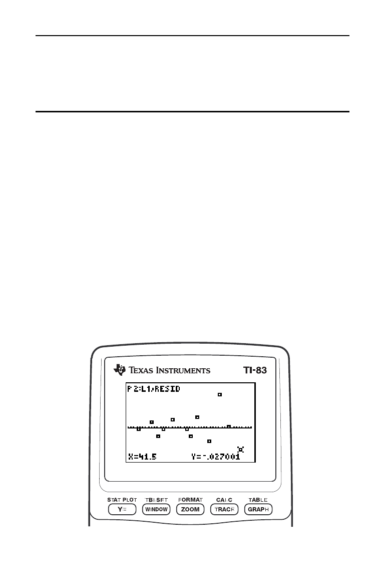
Statistics 12-1
8312STAT.DOC TI-83 international English Bob Fedorisko Revised: 02/19/01 12:42 PM Printed: 02/19/01 1:37
PM Page 1 of 38
12
Statistics
Getting Started: Pendulum Lengths and Periods
.........
12-2
Setting Up Statistical Analyses
...........................
12-10
Using the Stat List Editor
................................
12-11
Attaching Formulas to List Names
.......................
12-14
Detaching Formulas from List Names
....................
12-16
Switching Stat List Editor Contexts
......................
12-17
Stat List Editor Contexts
.................................
12-18
STAT EDIT
Menu
........................................
12-20
Regression Model Features
..............................
12-22
STAT CALC
Menu
........................................
12-24
Statistical Variables
......................................
12-29
Statistical Analysis in a Program
.........................
12-30
Statistical Plotting
.......................................
12-31
Statistical Plotting in a Program
.........................
12-37
Contents

12-2 Statistics
8312STAT.DOC TI-83 international English Bob Fedorisko Revised: 02/19/01 12:42 PM Printed: 02/19/01 1:37
PM Page 2 of 38
Getting Started is a fast-paced introduction. Read the chapter for details.
A group of students is attempting to determine the mathematical relationship
between the length of a pendulum and its period (one complete swing of a
pendulum). The group makes a simple pendulum from string and washers and
then suspends it from the ceiling. They record the pendulum’s period for each
of 12 string lengths.*
Length (cm) Time (sec)
6.5 0.51
11.0 0.68
13.2 0.73
15.0 0.79
18.0 0.88
23.1 0.99
24.4 1.01
26.6 1.08
30.5 1.13
34.3 1.26
37.6 1.28
41.5 1.32
1. Press
z
†
†
†
Í
to set
Func
graphing mode.
2. Press
…
5
to select
5:SetUpEditor
.
SetUpEditor
is pasted to the home
screen.
Press
Í
. This removes lists from stat
list editor columns
1
through
20
, and
then stores lists
L
1
through
L
6
in
columns
1
through
6
.
Note:
Removing lists from the stat list editor does not
delete them from memory.
3. Press
…
1
to select
1:Edit
from the
STAT EDIT
menu. The stat list editor is
displayed. If elements are stored in
L
1
and
L
2
, press
}
to move the cursor onto
L
1
, and then press
‘
Í
~
}
‘
Í
to clear both lists. Press
|
to move the rectangular cursor back to
the first row in
L
1
.
*This example is quoted and adapted from
Contemporary Precalculus Through Applications
,
by the North Carolina School of Science and Mathematics, by permission of Janson
Publications, Inc., Dedham, MA. 1-800-322-MATH. © 1992. All rights reserved.
Getting Started: Pendulum Lengths and Periods
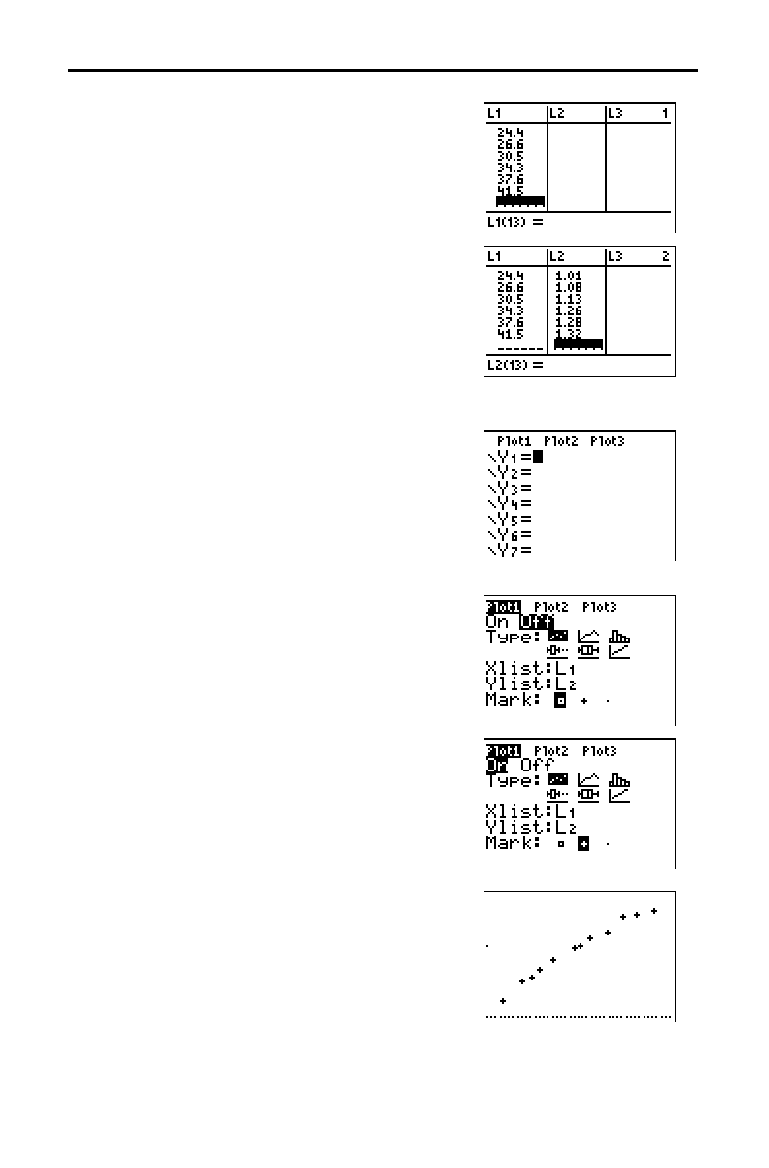
Statistics 12-3
8312STAT.DOC TI-83 international English Bob Fedorisko Revised: 02/19/01 12:42 PM Printed: 02/19/01 1:37
PM Page 3 of 38
4. Press 6
Ë
5
Í
to store the first
pendulum string length (6.5 cm) in
L
1
.
The rectangular cursor moves to the
next row. Repeat this step to enter each
of the 12 string length values in the table
on page 12
.
2.
5. Press
~
to move the rectangular cursor
to the first row in
L
2
.
Press
Ë
51
Í
to store the first time
measurement (.51 sec) in
L
2
. The
rectangular cursor moves to the next
row. Repeat this step to enter each of
the 12 time values in the table on
page 12
.
2.
6. Press
o
to display the
Y=
editor.
If necessary, press
‘
to clear the
function
Y
1
. As necessary, press
}
,
Í
,
and
~
to turn off
Plot1, Plot2, and Plot3
from the top line of the
Y=
editor
(Chapter 3). As necessary, press
†
,
|
,
and
Í
to deselect functions.
7. Press
y
[
STAT PLOT
] 1 to select 1:Plot1
from the
STAT PLOTS
menu. The stat
plot editor is displayed for plot 1.
8. Press
Í
to select On, which turns on
plot 1. Press
†
Í
to select
"
(scatter plot). Press
†
y
[
L1
] to
specify
Xlist:L
1
for plot 1. Press
†
y
[
L2
] to specify Ylist:L
2
for plot 1.
Press
†
~
Í
to select
+
as the Mark
for each data point on the scatter plot.
9. Press
q
9 to select 9:ZoomStat from
the
ZOOM
menu. The window variables
are adjusted automatically, and plot 1 is
displayed. This is a scatter plot of the
time-versus-length data.
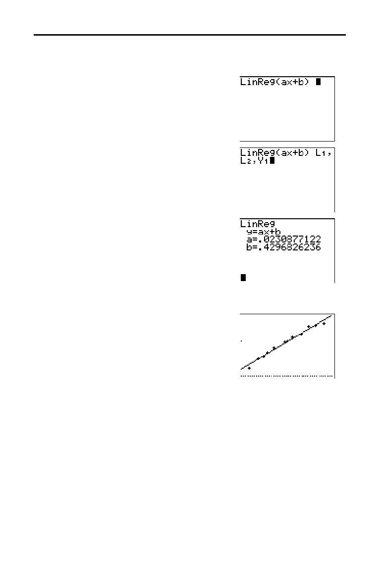
12-4 Statistics
8312STAT.DOC TI-83 international English Bob Fedorisko Revised: 02/19/01 12:42 PM Printed: 02/19/01 1:37
PM Page 4 of 38
Since the scatter plot of time-versus-length data appears to be approximately
linear, fit a line to the data.
10. Press
…
~
4 to select 4:LinReg(ax+b)
(linear regression model) from the
STAT
CALC
menu. LinReg(ax+b) is pasted to
the home screen.
11. Press
y
[
L1
]
¢
y
[
L2
]
¢
. Press
~
1 to display the
VARS Y
.
VARS
FUNCTION
secondary menu, and then
press
1 to select 1:Y
1
. L
1
, L
2
, and Y
1
are
pasted to the home screen as arguments
to
LinReg(ax+b).
12. Press
Í
to execute LinReg(ax+b). The
linear regression for the data in
L
1
and L
2
is calculated. Values for a and b are
displayed on the home screen. The linear
regression equation is stored in
Y
1
.
Residuals are calculated and stored
automatically in the list name
RESID,
which becomes an item on the
LIST
NAMES
menu.
13. Press
s
. The regression line and the
scatter plot are displayed.
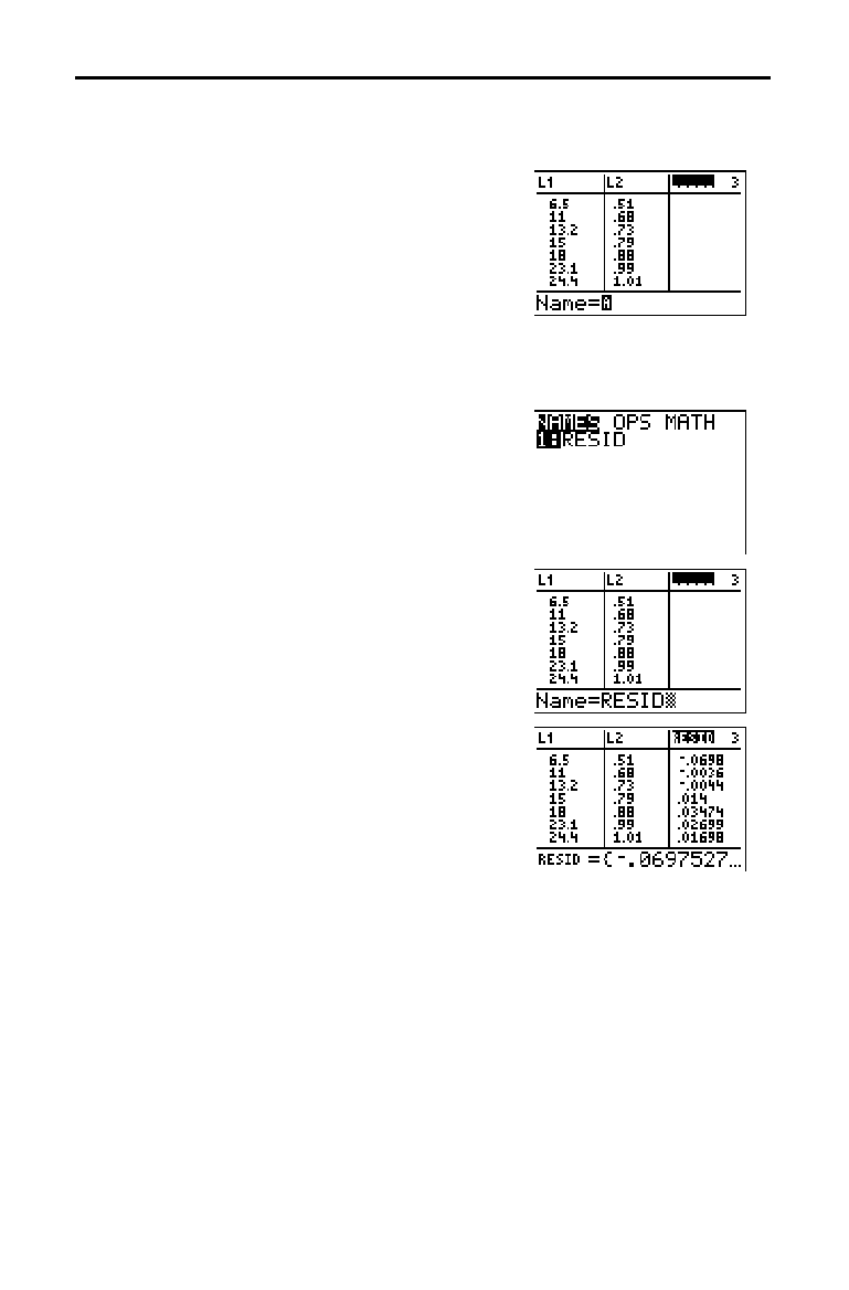
Statistics 12-5
8312STAT.DOC TI-83 international English Bob Fedorisko Revised: 02/19/01 12:42 PM Printed: 02/19/01 1:37
PM Page 5 of 38
The regression line appears to fit the central portion of the scatter plot well.
However, a residual plot may provide more information about this fit.
14. Press
…
1 to select 1:Edit. The stat
list editor is displayed.
Press
~
and
}
to move the cursor onto
L
3
.
Press
y
[
INS
]. An unnamed column is
displayed in column
3; L
3
, L
4
, L
5
, and L
6
shift right one column. The Name=
prompt is displayed in the entry line, and
alpha-lock is on.
15. Press
y
[
LIST
] to display the
LIST
NAMES
menu.
If necessary, press
†
to move the cursor
onto the list name
RESID.
16. Press
Í
to select RESID and paste it
to the stat list editor’s
Name= prompt.
17. Press
Í
. RESID is stored in column 3
of the stat list editor.
Press
†
repeatedly to examine the
residuals.
Notice that the first three residuals are negative. They correspond to the
shortest pendulum string lengths in
L
1
. The next five residuals are positive, and
three of the last four are negative. The latter correspond to the longer string
lengths in
L
1
. Plotting the residuals will show this pattern more clearly.
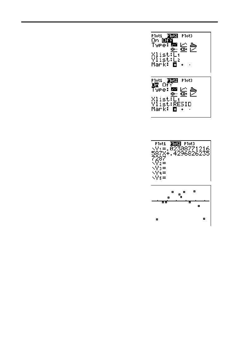
12-6 Statistics
8312STAT.DOC TI-83 international English Bob Fedorisko Revised: 02/19/01 12:42 PM Printed: 02/19/01 1:37
PM Page 6 of 38
18. Press
y
[
STAT PLOT
] 2 to select 2:Plot2
from the
STAT PLOTS
menu. The stat
plot editor is displayed for plot 2.
19. Press
Í
to select On, which turns on
plot 2.
Press
†
Í
to select
"
(scatter plot).
Press
†
y
[
L1
] to specify Xlist:L
1
for
plot 2. Press
†
[
R
] [
E
] [
S
] [
I
] [
D
]
(alpha-lock is on) to specify
Ylist:RESID
for plot 2. Press
†
Í
to select
›
as
the mark for each data point on the
scatter plot.
20. Press
o
to display the
Y=
editor.
Press
|
to move the cursor onto the
= sign, and then press
Í
to deselect
Y
1
. Press
}
Í
to turn off plot 1.
21. Press
q
9 to select 9:ZoomStat from
the
ZOOM
menu. The window variables
are adjusted automatically, and plot 2 is
displayed. This is a scatter plot of the
residuals.
Notice the pattern of the residuals: a group of negative residuals, then a group
of positive residuals, and then another group of negative residuals.
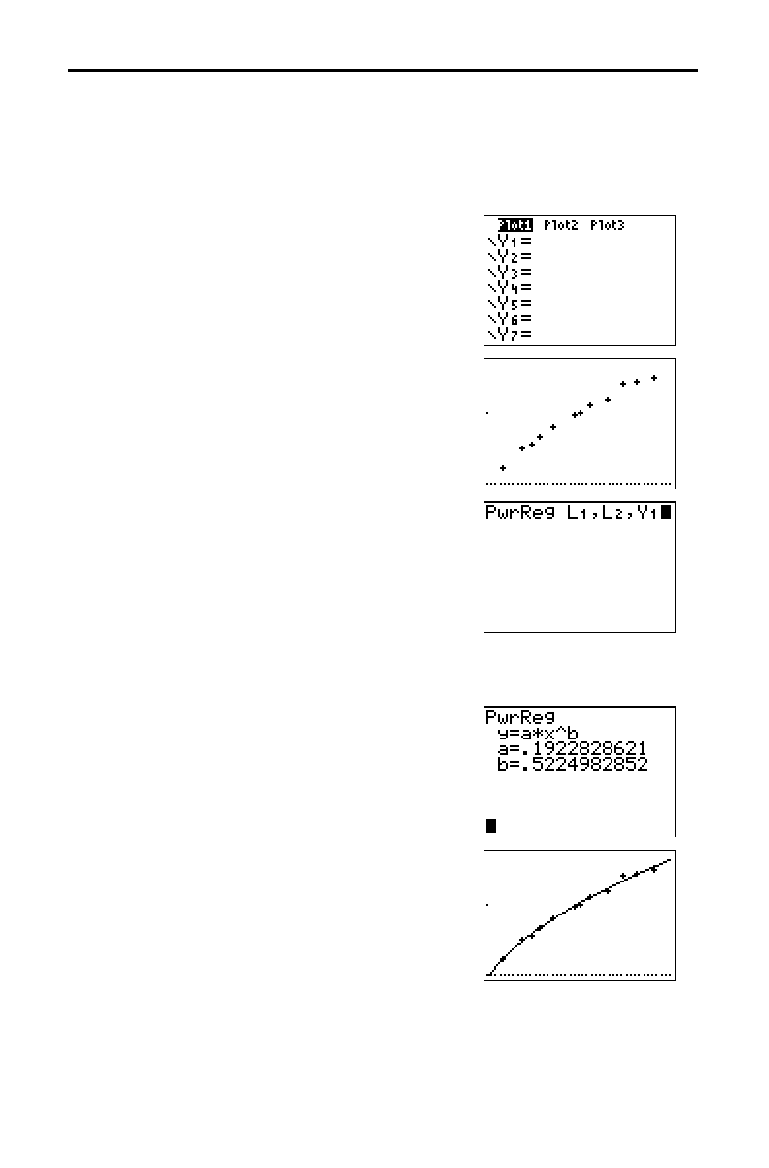
Statistics 12-7
8312STAT.DOC TI-83 international English Bob Fedorisko Revised: 02/19/01 12:42 PM Printed: 02/19/01 1:37
PM Page 7 of 38
The residual pattern indicates a curvature associated with this data set for
which the linear model did not account. The residual plot emphasizes a
downward curvature, so a model that curves down with the data would be
more accurate. Perhaps a function such as square root would fit. Try a power
regression to fit a function of the form y = a
ä
x
b
.
22. Press
o
to display the
Y=
editor.
Press
‘
to clear the linear regression
equation from
Y
1
. Press
}
Í
to turn
on plot 1. Press
~
Í
to turn off plot
2.
23. Press
q
9 to select 9:ZoomStat from
the
ZOOM
menu. The window variables
are adjusted automatically, and the
original scatter plot of time-versus-
length data (plot 1) is displayed.
24. Press
…
~
ƒ
[
A
] to select
A:PwrReg from the
STAT CALC
menu.
PwrReg is pasted to the home screen.
Press
y
[
L1
]
¢
y
[
L2
]
¢
. Press
~
1 to display the
VARS Y
.
VARS
FUNCTION
secondary menu, and then
press
1 to select 1:Y
1
. L
1
, L
2
, and Y
1
are
pasted to the home screen as arguments
to
PwrReg.
25. Press
Í
to calculate the power
regression. Values for
a and b are
displayed on the home screen. The
power regression equation is stored in
Y
1
. Residuals are calculated and stored
automatically in the list name
RESID.
26. Press
s
. The regression line and the
scatter plot are displayed.
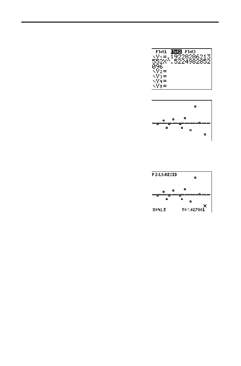
12-8 Statistics
8312STAT.DOC TI-83 international English Bob Fedorisko Revised: 02/19/01 12:42 PM Printed: 02/19/01 1:37
PM Page 8 of 38
The new function y=.192x
.522
appears to fit the data well. To get more
information, examine a residual plot.
27. Press
o
to display the
Y=
editor.
Press
|
Í
to deselect
Y
1
.
Press
}
Í
to turn off plot 1. Press
~
Í
to turn on plot 2.
Note:
Step 19 defined plot 2 to plot residuals (
RESID
)
versus string length (
L
1
).
28. Press
q
9 to select 9:ZoomStat from
the
ZOOM
menu. The window variables
are adjusted automatically, and plot 2 is
displayed. This is a scatter plot of the
residuals.
The new residual plot shows that the residuals are random in sign, with the
residuals increasing in magnitude as the string length increases.
To see the magnitudes of the residuals, continue with these steps.
29. Press
r
.
Press
~
and
|
to trace the data.
Observe the values for
Y at each point.
With this model, the largest positive
residual is about 0.041 and the smallest
negative residual is about
L
0.027. All
other residuals are less than 0.02 in
magnitude.
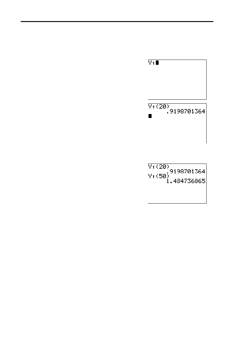
Statistics 12-9
8312STAT.DOC TI-83 international English Bob Fedorisko Revised: 02/19/01 12:42 PM Printed: 02/19/01 1:37
PM Page 9 of 38
Now that you have a good model for the relationship between length and
period, you can use the model to predict the period for a given string length.
To predict the periods for a pendulum with string lengths of 20 cm and 50 cm,
continue with these steps.
30. Press
~
1 to display the
VARS
Y
.
VARS FUNCTION
secondary menu, and
then press
1 to select 1:Y
1
. Y
1
is pasted
to the home screen.
31. Press
£
20
¤
to enter a string length of
20 cm.
Press
Í
to calculate the predicted
time of about 0.92 seconds.
Based on the residual analysis, we would
expect the prediction of about 0.92
seconds to be within about 0.02 seconds
of the actual value.
32. Press
y
[
ENTRY
] to recall the Last Entry.
Press
|
|
|
5 to change the string
length to 50 cm.
33. Press
Í
to calculate the predicted
time of about 1.48 seconds.
Since a string length of 50 cm exceeds
the lengths in the data set, and since
residuals appear to be increasing as
string length increases, we would expect
more error with this estimate.
Note:
You also can make predictions using the table
with the
TABLE SETUP
settings
Indpnt:Ask
and
Depend:Auto
(Chapter 7).
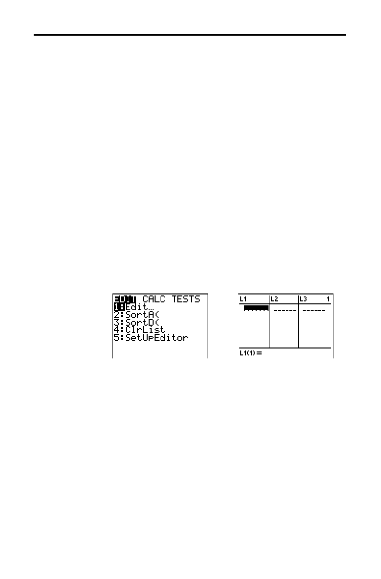
12-10 Statistics
8312STAT.DOC TI-83 international English Bob Fedorisko Revised: 02/19/01 12:42 PM Printed: 02/19/01 1:37
PM Page 10 of 38
Data for statistical analyses is stored in lists, which you
can create and edit using the stat list editor. The TI
-
83 has
six list variables in memory,
L
1
through L
6
, to which you
can store data for statistical calculations. Also, you can
store data to list names that you create (Chapter 11).
To set up a statistical analysis, follow these steps. Read the
chapter for details.
1. Enter the statistical data into one or more lists.
2. Plot the data.
3. Calculate the statistical variables or fit a model to the data.
4. Graph the regression equation for the plotted data.
5. Graph the residuals list for the given regression model.
The stat list editor is a table where you can store, edit, and
view up to 20 lists that are in memory. Also, you can create
list names from the stat list editor.
To display the stat list editor, press
…
, and then select
1:Edit from the
STAT EDIT
menu.
The top line displays list names. L
1
through L
6
are stored in
columns
1 through 6 after a memory reset. The number of
the current column is displayed in the top-right corner.
The bottom line is the entry line. All data entry occurs on
this line. The characteristics of this line change according
to the current context (page 12
.
17).
The center area displays up to seven elements of up to
three lists; it abbreviates values when necessary. The entry
line displays the full value of the current element.
Setting Up Statistical Analyses
Using Lists to
Store Data
Setting Up a
Statistical
Analysis
Displaying the
Stat List Editor
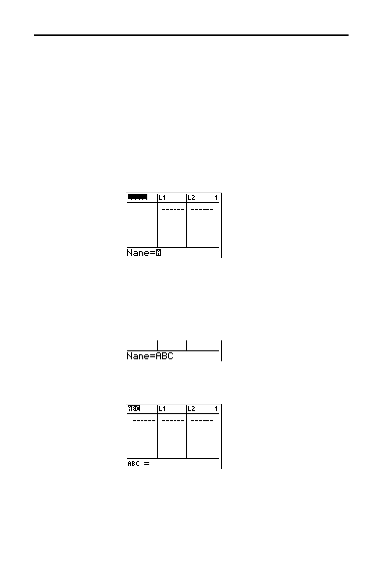
Statistics 12-11
8312STAT.DOC TI-83 international English Bob Fedorisko Revised: 02/19/01 12:42 PM Printed: 02/19/01 1:37
PM Page 11 of 38
To enter a list name in the stat list editor, follow these steps.
1. Display the
Name= prompt in the entry line in either of
two ways.
•
Move the cursor onto the list name in the column
where you want to insert a list, and then press
y
[
INS
]. An unnamed column is displayed and the
remaining lists shift right one column.
•
Press
}
until the cursor is on the top line, and then
press
~
until you reach the unnamed column.
Note:
If list names are stored to all 20 columns, you must remove
a list name to make room for an unnamed column.
The Name= prompt is displayed and alpha-lock is on.
2. Enter a valid list name in any of four ways.
•
Select a name from the
LIST NAMES
menu (Chapter 11).
•
Enter
L
1
, L
2
, L
3
, L
4
, L
5
, or L
6
from the keyboard.
•
Enter an existing user-created list name directly from
the keyboard.
•
Enter a new user-created list name (page 12
.
12).
3. Press
Í
or
†
to store the list name and its
elements, if any, in the current column of the stat list
editor.
To begin entering, scrolling, or editing list elements, press
†
. The rectangular cursor is displayed.
Note:
If the list name you entered in step 2 already was stored in
another stat list editor column, then the list and its elements, if any,
move to the current column from the previous column. Remaining list
names shift accordingly.
Using the Stat List Editor
Entering a List
Name in the Stat
List Editor

12-12 Statistics
8312STAT.DOC TI-83 international English Bob Fedorisko Revised: 02/19/01 12:42 PM Printed: 02/19/01 1:37
PM Page 12 of 38
To create a name in the stat list editor, follow these steps.
1. Follow step 1 on page 12
.
11 to display the
Name=
prompt.
2. Press [
letter from A to Z or
q
] to enter the first letter of
the name. The first character cannot be a number.
3. Enter zero to four letters,
q
, or numbers to complete the
new user-created list name. List names can be one to
five characters long.
4. Press
Í
or
†
to store the list name in the current
column of the stat list editor. The list name becomes an
item on the
LIST NAMES
menu (Chapter 11).
To remove a list from the stat list editor, move the cursor
onto the list name and then press
{
. The list is not deleted
from memory; it is only removed from the stat list editor.
Note:
To delete a list name from memory, use the
MEMORY
DELETE:List
selection screen (Chapter 18).
You can remove all user-created lists from the stat list
editor and restore list names
L
1
through L
6
to columns 1
through 6 in either of two ways.
•
Use
SetUpEditor with no arguments (page 12
.
21).
•
Reset all memory (Chapter 18).
You can clear all elements from a list in any of five ways.
•
Use
ClrList to clear specified lists (page 12
.
20).
•
In the stat list editor, press
}
to move the cursor onto a
list name, and then press
‘
Í
.
•
In the stat list editor, move the cursor onto each
element, and then press
{
one by one.
•
On the home screen or in the program editor, enter
0
!
dim(
listname
) to set the dimension of
listname
to 0
(Chapter 11).
•
Use
ClrAllLists to clear all lists in memory (Chapter 18).
Creating a Name
in the Stat List
Editor
Removing a List
from the Stat List
Editor
Removing All
Lists and
Restoring L
1
through L
6
Clearing All
Elements from a
List
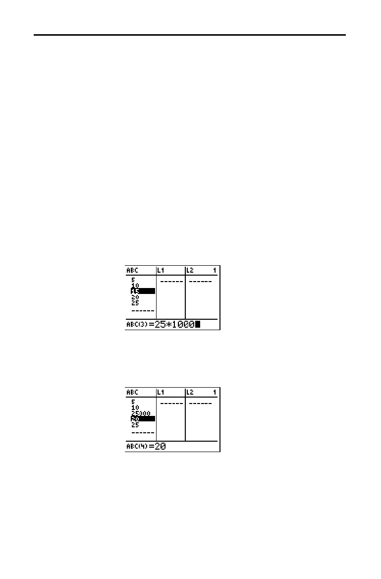
Statistics 12-13
8312STAT.DOC TI-83 international English Bob Fedorisko Revised: 02/19/01 12:42 PM Printed: 02/19/01 1:37
PM Page 13 of 38
To edit a list element, follow these steps.
1. Move the rectangular cursor onto the element you want
to edit.
2. Press
Í
to move the cursor to the entry line.
Note:
If you want to replace the current value, you can enter a new
value without first pressing
Í
. When you enter the first
character, the current value is cleared automatically.
3. Edit the element in the entry line.
•
Press one or more keys to enter the new value. When
you enter the first character, the current value is
cleared automatically.
•
Press
~
to move the cursor to the character before
which you want to insert, press
y
[
INS
], and then
enter one or more characters.
•
Press
~
to move the cursor to a character you want to
delete, and then press
{
to delete the character.
To cancel any editing and restore the original element at
the rectangular cursor, press
‘
Í
.
Note:
You can enter expressions and variables for elements.
4. Press
Í
,
}
, or
†
to update the list. If you entered
an expression, it is evaluated. If you entered only a
variable, the stored value is displayed as a list element.
When you edit a list element in the stat list editor, the list is
updated in memory immediately.
Editing a List
Element
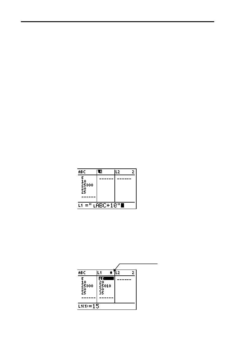
12-14 Statistics
8312STAT.DOC TI-83 international English Bob Fedorisko Revised: 02/19/01 12:42 PM Printed: 02/19/01 1:37
PM Page 14 of 38
You can attach a formula to a list name in the stat list
editor, and then display and edit the calculated list
elements. When executed, the attached formula must
resolve to a list. Chapter 11 describes in detail the concept
of attaching formulas to list names.
To attach a formula to a list name that is stored in the stat
list editor, follow these steps.
1. Press
…
Í
to display the stat list editor.
2. Press
}
to move the cursor to the top line.
3. Press
|
or
~
, if necessary, to move the cursor onto the
list name to which you want to attach the formula.
Note:
If a formula in quotation marks is displayed on the entry line,
then a formula is already attached to the list name. To edit the
formula, press
Í
, and then edit the formula.
4. Press
ƒ
[
ã
], enter the formula, and press
ƒ
[
ã
].
Note:
If you do not use quotation marks, the TI
-
83 calculates and
displays the same initial list of answers, but does not attach the
formula for future calculations.
Note:
Any user-created list name referenced in a formula must be
preceded by an
Ù
symbol (Chapter 11).
5. Press
Í
. The TI
-
83 calculates each list element and
stores it to the list name to which the formula is
attached. A lock symbol is displayed in the stat list
editor, next to the list name to which the formula is
attached.
Attaching Formulas to List Names
Attaching a
Formula to a List
Name in Stat List
Editor
lock symbol
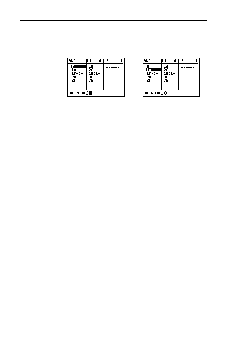
Statistics 12-15
8312STAT.DOC TI-83 international English Bob Fedorisko Revised: 02/19/01 12:42 PM Printed: 02/19/01 1:37
PM Page 15 of 38
When you edit an element of a list referenced in an
attached formula, the TI
-
83 updates the corresponding
element in the list to which the formula is attached
(Chapter 11).
When a list with a formula attached is displayed in the stat
list editor and you edit or enter elements of another
displayed list, then the TI
-
83 takes slightly longer to accept
each edit or entry than when no lists with formulas
attached are in view.
Tip:
To speed editing time, scroll horizontally until no lists with
formulas are displayed, or rearrange the stat list editor so that no lists
with formulas are displayed.
On the home screen, you can attach to a list a formula that
references another list with dimension 0 (Chapter 11).
However, you cannot display the formula-generated list in
the stat list editor or on the home screen until you enter at
least one element to the list that the formula references.
All elements of a list referenced by an attached formula
must be valid for the attached formula. For example, if
Real
number mode is set and the attached formula is
log(L
1
)
, then each element of
L
1
must be greater than 0,
since the logarithm of a negative number returns a
complex result.
Tip:
If an error menu is returned when you attempt to display a
formula-generated list in the stat list editor, you can select
2:Goto
,
write down the formula that is attached to the list, and then press
‘
Í
to detach (clear) the formula. You then can use the stat
list editor to find the source of the error. After making the appropriate
changes, you can reattach the formula to a list.
If you do not want to clear the formula, you can select
1:Quit
, display
the referenced list on the home screen, and find and edit the source of
the error. To edit an element of a list on the home screen, store the
new value to
listname
(
element#
)
(Chapter 11).
Using the Stat
List Editor When
Formula-
Generated Lists
Are Displayed
Handling Errors
Resulting from
Attached
Formulas

12-16 Statistics
8312STAT.DOC TI-83 international English Bob Fedorisko Revised: 02/19/01 12:42 PM Printed: 02/19/01 1:37
PM Page 16 of 38
You can detach (clear) a formula from a list name in any of
four ways.
•
In the stat list editor, move the cursor onto the name of
the list to which a formula is attached. Press
Í
‘
Í
. All list elements remain, but the formula
is detached and the lock symbol disappears.
•
In the stat list editor, move the cursor onto an element
of the list to which a formula is attached. Press
Í
,
edit the element, and then press
Í
. The element
changes, the formula is detached, and the lock symbol
disappears. All other list elements remain.
•
Use
ClrList (page 12
.
20). All elements of one or more
specified lists are cleared, each formula is detached, and
each lock symbol disappears. All list names remain.
•
Use
ClrAllLists (Chapter 18). All elements of all lists in
memory are cleared, all formulas are detached from all
list names, and all lock symbols disappear. All list
names remain.
As described above, one way to detach a formula from a
list name is to edit an element of the list to which the
formula is attached. The TI
-
83 protects against
inadvertently detaching the formula from the list name by
editing an element of the formula-generated list.
Because of the protection feature, you must press
Í
before you can edit an element of a formula-generated list.
The protection feature does not allow you to delete an
element of a list to which a formula is attached. To delete
an element of a list to which a formula is attached, you
must first detach the formula in any of the ways described
above.
Detaching Formulas from List Names
Detaching a
Formula from a
List Name
Editing an
Element of a
Formula-
Generated List
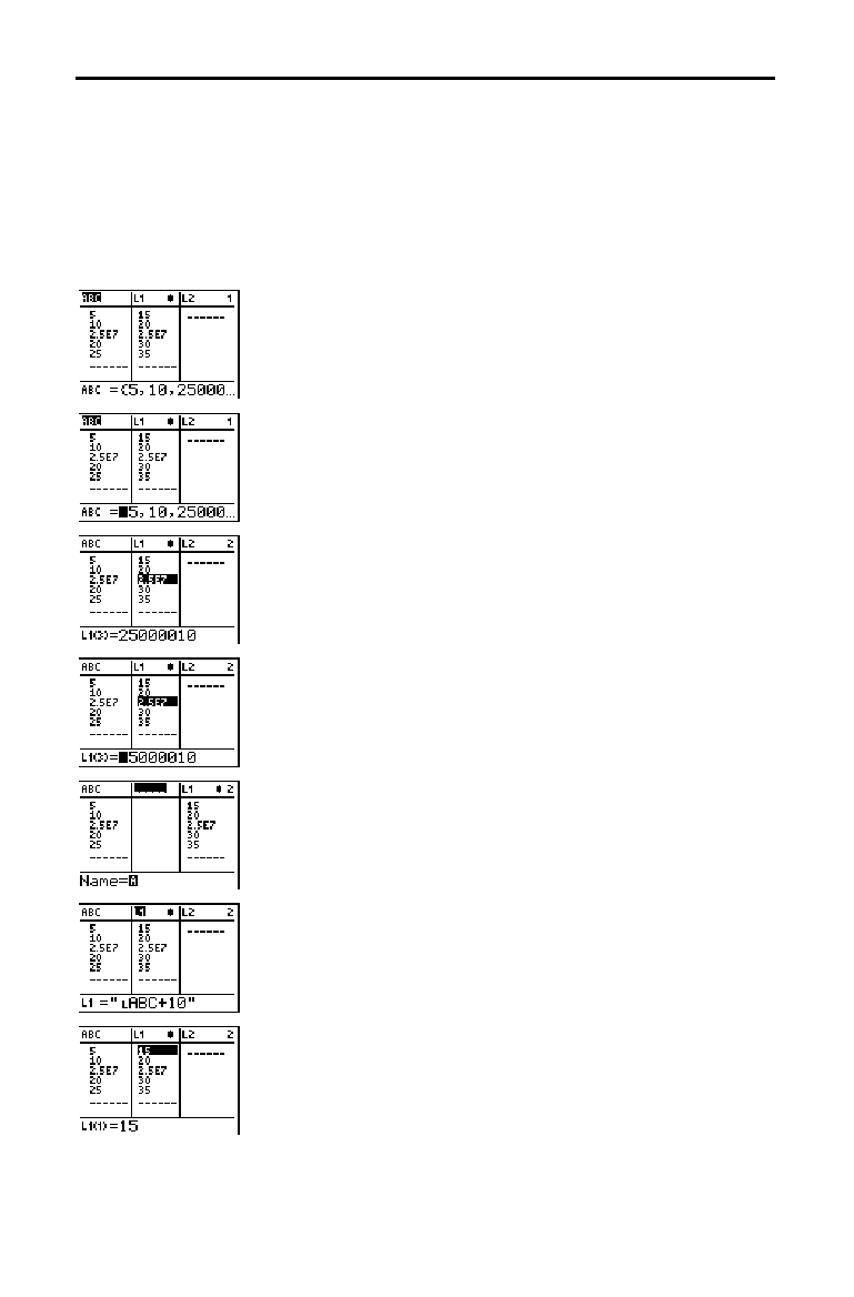
Statistics 12-17
8312STAT.DOC TI-83 international English Bob Fedorisko Revised: 02/19/01 12:42 PM Printed: 02/19/01 1:37
PM Page 17 of 38
The stat list editor has four contexts.
•
View-elements context
•
Edit-elements context
•
View-names context
•
Enter-name context
The stat list editor is first displayed in view-elements
context. To switch through the four contexts, select
1:Edit
from the
STAT EDIT
menu and follow these steps.
1. Press
}
to move the cursor onto a list name. You are
now in view-names context. Press
~
and
|
to view list
names stored in other stat list editor columns.
2. Press
Í
. You are now in edit-elements context. You
may edit any element in a list. All elements of the
current list are displayed in braces (
{ } )in the entry
line. Press
~
and
|
to view more list elements.
3. Press
Í
again. You are now in view-elements
context. Press
~
,
|
,
†
, and
}
to view other list
elements. The current element’s full value is displayed
in the entry line.
4. Press
Í
again. You are now in edit-elements
context. You may edit the current element in the entry
line.
5. Press
}
until the cursor is on a list name, then press
y
[
INS
]. You are now in enter-name context.
6. Press
‘
. You are now in view-names context.
7. Press
†
. You are now back in view-elements context.
Switching Stat List Editor Contexts
Stat List Editor
Contexts
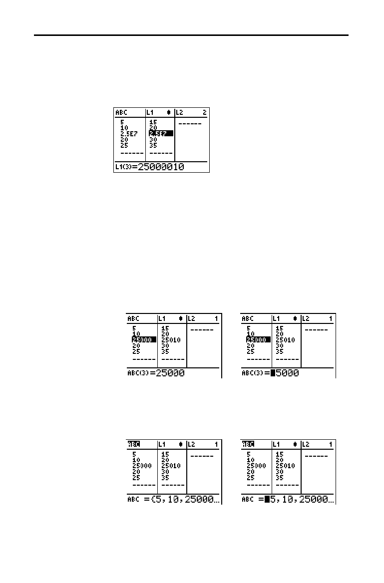
12-18 Statistics
8312STAT.DOC TI-83 international English Bob Fedorisko Revised: 02/19/01 12:42 PM Printed: 02/19/01 1:37
PM Page 18 of 38
In view-elements context, the entry line displays the list
name, the current element’s place in that list, and the full
value of the current element, up to 12 characters at a time.
An ellipsis (
...) indicates that the element continues beyond
12 characters.
To page down the list six elements, press
ƒ
†
. To
page up six elements, press
ƒ
}
. To delete a list
element, press
{
. Remaining elements shift up one row.
To insert a new element, press
y
[
INS
]. 0 is the default
value for a new element.
In edit-elements context, the data displayed in the entry
line depends on the previous context.
•
When you switch to edit-elements context from view-
elements context, the full value of the current element
is displayed. You can edit the value of this element, and
then press
†
and
}
to edit other list elements.
&
•
When you switch to edit-elements context from view-
names context, the full values of all elements in the list
are displayed. An ellipsis indicates that list elements
continue beyond the screen. You can press
~
and
|
to
edit any element in the list.
&
Note:
In edit-elements context, you can attach a formula to a list
name only if you switched to it from view-names context.
Stat List Editor Contexts
View-Elements
Context
Edit-Elements
Context
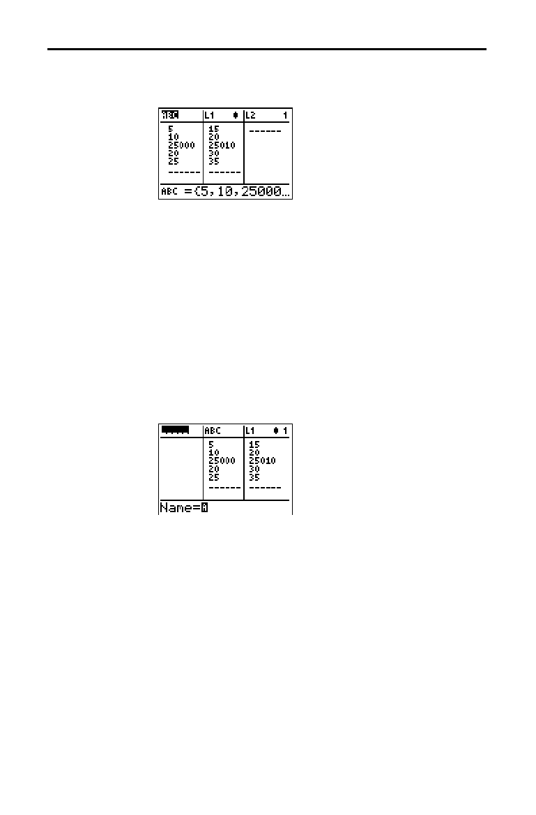
Statistics 12-19
8312STAT.DOC TI-83 international English Bob Fedorisko Revised: 02/19/01 12:42 PM Printed: 02/19/01 1:37
PM Page 19 of 38
In view-names context, the entry line displays the list name
and the list elements.
To remove a list from the stat list editor, press
{
.
Remaining lists shift to the left one column. The list is not
deleted from memory.
To insert a name in the current column, press
y
[
INS
].
Remaining columns shift to the right one column.
In enter-name context, the
Name= prompt is displayed in
the entry line, and alpha-lock is on.
At the
Name= prompt, you can create a new list name,
paste a list name from
L
1
to L
6
from the keyboard, or paste
an existing list name from the
LIST NAMES
menu
(Chapter 11). The
Ù
symbol is not required at the Name=
prompt.
To leave enter-name context without entering a list name,
press
‘
. The stat list editor switches to view-names
context.
View-Names
Context
Enter-Name
Context
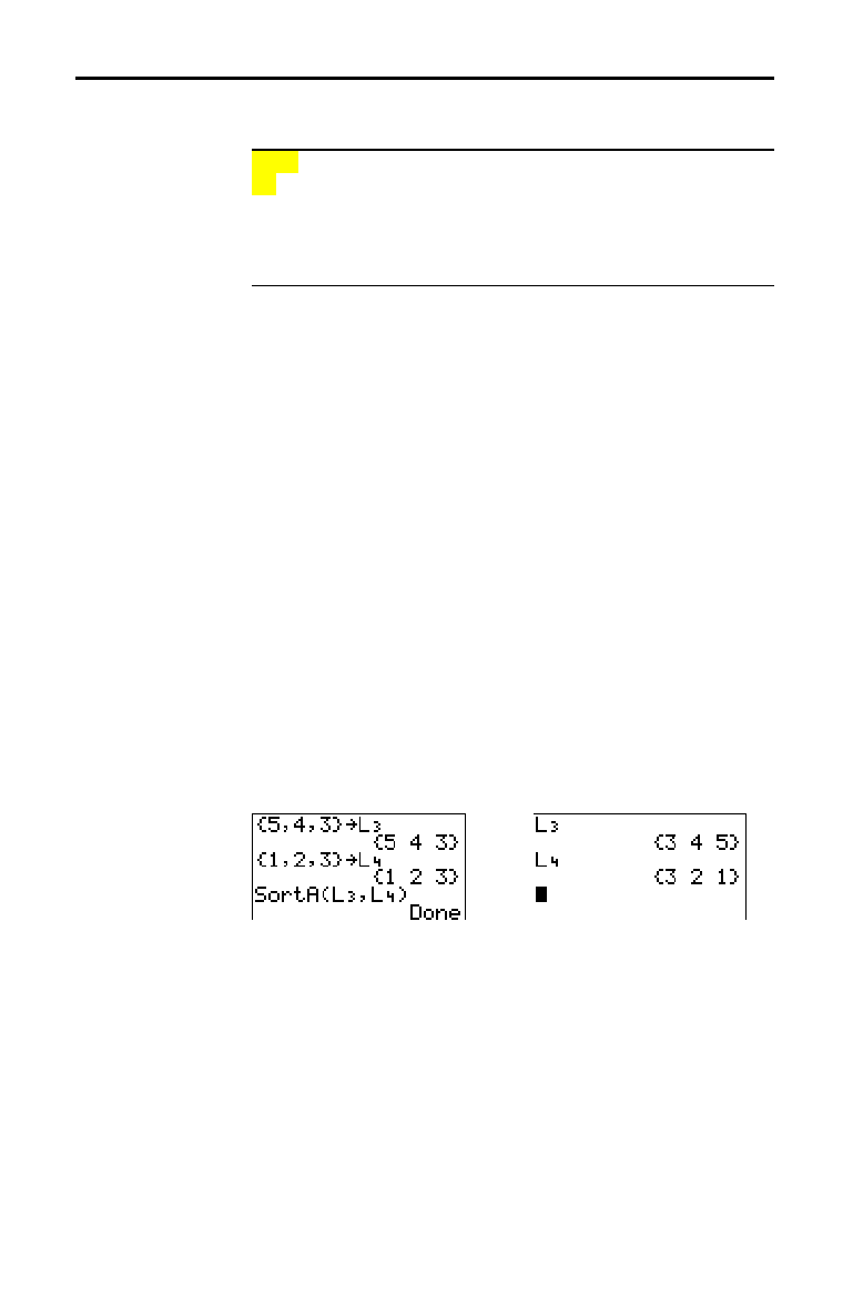
12-20 Statistics
8312STAT.DOC TI-83 international English Bob Fedorisko Revised: 02/19/01 12:42 PM Printed: 02/19/01 1:37
PM Page 20 of 38
To display the
STAT EDIT
menu, press
…
.
EDIT CALC TESTS
1: Edit
...
Displays the stat list editor.
2: SortA(
Sorts a list in ascending order.
3: SortD(
Sorts a list in descending order.
4: ClrList
Deletes all elements of a list.
5: SetUpEditor
Stores lists in the stat list editor.
Note:
Chapter 13: Inferential Statistics describes the
STAT TESTS
menu items.
SortA(
(sort ascending) sorts list elements from low to high
values.
SortD(
(sort descending) sorts list elements from
high to low values. Complex lists are sorted based on
magnitude (modulus).
SortA(
and
SortD(
each can sort in
either of two ways.
•
With one
listname
,
SortA(
and
SortD(
sort the elements
in
listname
and update the list in memory.
•
With two or more lists,
SortA(
and
SortD(
sort
keylistname
, and then sort each
dependlist
by placing
its elements in the same order as the corresponding
elements in
keylistname
. This lets you sort two-variable
data on
X
and keep the data pairs together. All lists
must have the same dimension.
The sorted lists are updated in memory.
SortA(
listname
)
SortD(
listname
)
SortA(
keylistname
,
dependlist1
[
,
dependlist2
,
...
,
dependlist n
]
)
SortD(
keylistname
,
dependlist1
[
,
dependlist2
,
...
,
dependlist n
]
)
Note:
SortA(
and
SortD(
are the same as
SortA(
and
SortD(
on the
LIST OPS
menu.
ClrList
clears (deletes) from memory the elements of one
or more
listnames
.
ClrList
also detaches any formula
attached to a
listname
.
ClrList
listname1
,
listname2
,
...
,
listname n
Note:
To clear from memory all elements of all list names, use
ClrAllLists
(Chapter 18).
STAT EDIT Menu
STAT EDIT Menu
SortA(, SortD(
ClrList
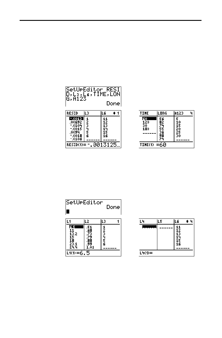
Statistics 12-21
8312STAT.DOC TI-83 international English Bob Fedorisko Revised: 02/19/01 12:42 PM Printed: 02/19/01 1:37
PM Page 21 of 38
With SetUpEditor you can set up the stat list editor to
display one or more
listnames
in the order that you
specify. You can specify zero to 20
listnames
.
SetUpEditor [
listname1
,
listname2
,...,
listname n
]
SetUpEditor with one to 20
listnames
removes all list
names from the stat list editor and then stores
listnames
in
the stat list editor columns in the specified order,
beginning in column
1.
If you enter a
listname
that is not stored in memory
already, then
listname
is created and stored in memory; it
becomes an item on the
LIST NAMES
menu.
SetUpEditor with no
listnames
removes all list names from
the stat list editor and restores list names
L
1
through L
6
in
the stat list editor columns
1 through 6.
SetUpEditor
Restoring L
1
through L
6
to the
Stat List Editor
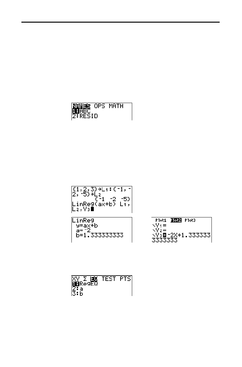
12-22 Statistics
8312STAT.DOC TI-83 international English Bob Fedorisko Revised: 02/19/01 12:42 PM Printed: 02/19/01 1:37
PM Page 22 of 38
STAT CALC
menu items 3 through C are regression models
(page 12
.
24). The automatic residual list and automatic
regression equation features apply to all regression
models. Diagnostics display mode applies to some
regression models.
When you execute a regression model, the automatic
residual list feature computes and stores the residuals to
the list name
RESID. RESID becomes an item on the
LIST NAMES
menu (Chapter 11).
The TI
-
83 uses the formula below to compute RESID list
elements. The next section describes the variable
RegEQ.
RESID =
Ylistname
N
RegEQ(
Xlistname
)
Each regression model has an optional argument,
regequ
, for
which you can specify a
Y=
variable such as Y
1
. Upon
execution, the regression equation is stored automatically to
the specified
Y=
variable and the
Y=
function is selected.
Regardless of whether you specify a
Y=
variable for
regequ
,
the regression equation always is stored to the TI
-
83
variable
RegEQ, which is item 1 on the
VARS Statistics EQ
secondary menu.
Note:
For the regression equation, you can use the fixed-decimal
mode setting to control the number of digits stored after the decimal
point (Chapter 1). However, limiting the number of digits to a small
number could affect the accuracy of the fit.
Regression Model Features
Regression
Model Features
Automatic
Residual List
Automatic
Regression
Equation

Statistics 12-23
8312STAT.DOC TI-83 international English Bob Fedorisko Revised: 02/19/01 12:42 PM Printed: 02/19/01 1:37
PM Page 23 of 38
When you execute some regression models, the TI
-
83
computes and stores diagnostics values for
r (correlation
coefficient) and
r
2
(coefficient of determination) or for R
2
(coefficient of determination).
r and r
2
are computed and stored for these regression
models.
LinReg(ax+b) LnReg PwrReg
LinReg(a+bx) ExpReg
R
2
is computed and stored for these regression models.
QuadReg CubicReg QuartReg
The r and r
2
that are computed for LnReg, ExpReg, and
PwrReg are based on the linearly transformed data. For
example, for
ExpReg (y=ab^x), r and r
2
are computed on
ln y=ln a+x(ln b).
By default, these values are not displayed with the results
of a regression model when you execute it. However, you
can set the diagnostics display mode by executing the
DiagnosticOn or DiagnosticOff instruction. Each instruction
is in the
CATALOG
(Chapter 15).
Note:
To set
DiagnosticOn
or
DiagnosticOff
from the home
screen, press
y
[
CATALOG
], and then select the instruction for the
mode you want. The instruction is pasted to the home screen. Press
Í
to set the mode.
When DiagnosticOn is set, diagnostics are displayed with
the results when you execute a regression model.
When DiagnosticOff is set, diagnostics are not displayed
with the results when you execute a regression model.
Diagnostics
Display Mode

12-24 Statistics
8312STAT.DOC TI-83 international English Bob Fedorisko Revised: 02/19/01 12:42 PM Printed: 02/19/01 1:37
PM Page 24 of 38
To display the
STAT CALC
menu, press
…
~
.
EDIT CALC TESTS
1: 1-Var Stats
Calculates 1-variable statistics.
2: 2-Var Stats
Calculates 2-variable statistics.
3: Med-Med
Calculates a median-median line.
4: LinReg(ax+b)
Fits a linear model to data.
5: QuadReg
Fits a quadratic model to data.
6: CubicReg
Fits a cubic model to data.
7: QuartReg
Fits a quartic model to data.
8: LinReg(a+bx)
Fits a linear model to data.
9: LnReg
Fits a logarithmic model to data.
0: ExpReg
Fits an exponential model to data.
A: PwrReg
Fits a power model to data.
B: Logistic
Fits a logistic model to data.
C: SinReg
Fits a sinusoidal model to data.
For each
STAT CALC
menu item, if neither
Xlistname
nor
Ylistname
is specified, then the default list names are
L
1
and L
2
. If you do not specify
freqlist
, then the default is 1
occurrence of each list element.
For most
STAT CALC
menu items, you can specify a list of
data occurrences, or frequencies (
freqlist
).
Each element in
freqlist
indicates how many times the
corresponding data point or data pair occurs in the data set
you are analyzing.
For example, if
L
1
={15,12,9,14} and
Ù
FREQ={1,4,1,3}
, then
the TI
-
83 interprets the instruction
1
.
Var Stats L
1
,
Ù
FREQ
to
mean that
15 occurs once, 12 occurs four times, 9 occurs
once, and
14 occurs three times.
Each element in
freqlist
must be
‚
0, and at least one
element must be > 0.
Noninteger
freqlist
elements are valid. This is useful when
entering frequencies expressed as percentages or parts
that add up to 1. However, if
freqlist
contains noninteger
frequencies,
Sx and Sy are undefined; values are not
displayed for
Sx and Sy in the statistical results.
STAT CALC Menu
STAT CALC
Menu
Frequency of
Occurrence for
Data Points
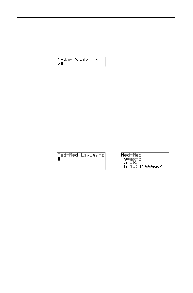
Statistics 12-25
8312STAT.DOC TI-83 international English Bob Fedorisko Revised: 02/19/01 12:42 PM Printed: 02/19/01 1:37
PM Page 25 of 38
1
.
Var Stats (one-variable statistics) analyzes data with one
measured variable. Each element in
freqlist
is the
frequency of occurrence for each corresponding data point
in
Xlistname
.
freqlist
elements must be real numbers > 0.
1
.
Var Stats [
Xlistname
,
freqlist
]
2
.
Var Stats (two-variable statistics) analyzes paired data.
Xlistname
is the independent variable.
Ylistname
is the
dependent variable. Each element in
freqlist
is the
frequency of occurrence for each data pair
(
Xlistname,Ylistname
).
2
.
Var Stats [
Xlistname
,
Ylistname
,
freqlist
]
Med
.
Med (median-median) fits the model equation y=ax+b
to the data using the median-median line (resistant line)
technique, calculating the summary points
x
1
, y
1
, x
2
, y
2
, x
3
,
and
y
3
. Med
.
Med displays values for a (slope) and
b (y-intercept).
Med
.
Med [
Xlistname
,
Ylistname
,
freqlist
,
regequ
]
LinReg(ax+b) (linear regression) fits the model equation
y=ax+b to the data using a least-squares fit. It displays values
for
a (slope) and b (y-intercept); when DiagnosticOn is set, it
also displays values for
r
2
and r.
LinReg(ax+b) [
Xlistname
,
Ylistname
,
freqlist
,
regequ
]
QuadReg (quadratic regression) fits the second-degree
polynomial y=ax
2
+bx+c to the data. It displays values for a,
b, and c; when DiagnosticOn is set, it also displays a value
for
R
2
. For three data points, the equation is a polynomial
fit; for four or more, it is a polynomial regression. At least
three data points are required.
QuadReg [
Xlistname
,
Ylistname
,
freqlist
,
regequ
]
1-Var Stats
2-Var Stats
Med-Med
(ax+b)
LinReg
(ax+b)
QuadReg
(ax
2
+bx+c)

12-26 Statistics
8312STAT.DOC TI-83 international English Bob Fedorisko Revised: 02/19/01 12:42 PM Printed: 02/19/01 1:37
PM Page 26 of 38
CubicReg (cubic regression) fits the third-degree
polynomial y=ax
3
+bx
2
+cx+d to the data. It displays values
for
a, b, c, and d; when DiagnosticOn is set, it also displays
a value for
R
2
. For four points, the equation is a polynomial
fit; for five or more, it is a polynomial regression. At least
four points are required.
CubicReg [
Xlistname
,
Ylistname
,
freqlist
,
regequ
]
QuartReg (quartic regression) fits the fourth-degree
polynomial y=ax
4
+bx
3
+cx
2
+dx+e to the data. It displays
values for
a, b, c, d, and e; when DiagnosticOn is set, it also
displays a value for
R
2
. For five points, the equation is a
polynomial fit; for six or more, it is a polynomial
regression. At least five points are required.
QuartReg [
Xlistname
,
Ylistname
,
freqlist
,
regequ
]
LinReg(a+bx) (linear regression) fits the model equation
y=a+bx to the data using a least-squares fit. It displays values
for
a (y-intercept) and b (slope); when DiagnosticOn is set, it
also displays values for
r
2
and r.
LinReg(a+bx) [
Xlistname
,
Ylistname
,
freqlist
,
regequ
]
LnReg (logarithmic regression) fits the model equation
y=a+b ln(x) to the data using a least-squares fit and
transformed values ln(x) and y. It displays values for
a and
b; when DiagnosticOn is set, it also displays values for r
2
and r.
LnReg [
Xlistname
,
Ylistname
,
freqlist
,
regequ
]
ExpReg (exponential regression) fits the model equation
y=ab
x
to the data using a least-squares fit and transformed
values x and ln(y). It displays values for
a and b; when
DiagnosticOn is set, it also displays values for r
2
and r.
ExpReg [
Xlistname
,
Ylistname
,
freqlist
,
regequ
]
CubicReg
(ax
3
+bx
2
+cx+d)
QuartReg
(ax
4
+bx
3
+cx
2
+
dx+e)
LinReg
(a+bx)
LnReg
(a+b ln(x))
ExpReg
(ab
x
)

Statistics 12-27
8312STAT.DOC TI-83 international English Bob Fedorisko Revised: 02/19/01 12:42 PM Printed: 02/19/01 1:37
PM Page 27 of 38
PwrReg (power regression) fits the model equation y=ax
b
to
the data using a least-squares fit and transformed values
ln(x) and ln(y). It displays values for
a and b; when
DiagnosticOn is set, it also displays values for r
2
and r.
PwrReg [
Xlistname
,
Ylistname
,
freqlist
,
regequ
]
Logistic fits the model equation y=c / (1+a
ä
e
L
bx
) to the data
using an iterative least-squares fit. It displays values for
a, b,
and
c.
Logistic [
Xlistname
,
Ylistname
,
freqlist
,
regequ
]
SinReg (sinusoidal regression) fits the model equation
y=a sin(bx+c)+d to the data using an iterative least-squares
fit. It displays values for
a, b, c, and d. At least four data
points are required. At least two data points per cycle are
required in order to avoid aliased frequency estimates.
SinReg [
iterations
,
Xlistname
,
Ylistname
,
period
,
regequ
]
iterations
is the maximum number of times the algorithm
will iterate to find a solution. The value for
iterations
can
be an integer
‚
1 and
16; if not specified, the default is 3.
The algorithm may find a solution before
iterations
is
reached. Typically, larger values for
iterations
result in
longer execution times and better accuracy for
SinReg, and
vice versa.
A
period
guess is optional. If you do not specify
period
, the
difference between time values in
Xlistname
must be equal
and the time values must be ordered in ascending
sequential order. If you specify
period
, the algorithm may
find a solution more quickly, or it may find a solution when
it would not have found one if you had omitted a value for
period
. If you specify
period
, the differences between time
values in
Xlistname
can be unequal.
Note:
The output of
SinReg
is always in radians, regardless of the
Radian/Degree
mode setting.
A SinReg example is shown on the next page.
PwrReg
(ax
b
)
Logistic
c/(1+a
ä
e
L
bx
)
SinReg
a sin(bx+c)+d
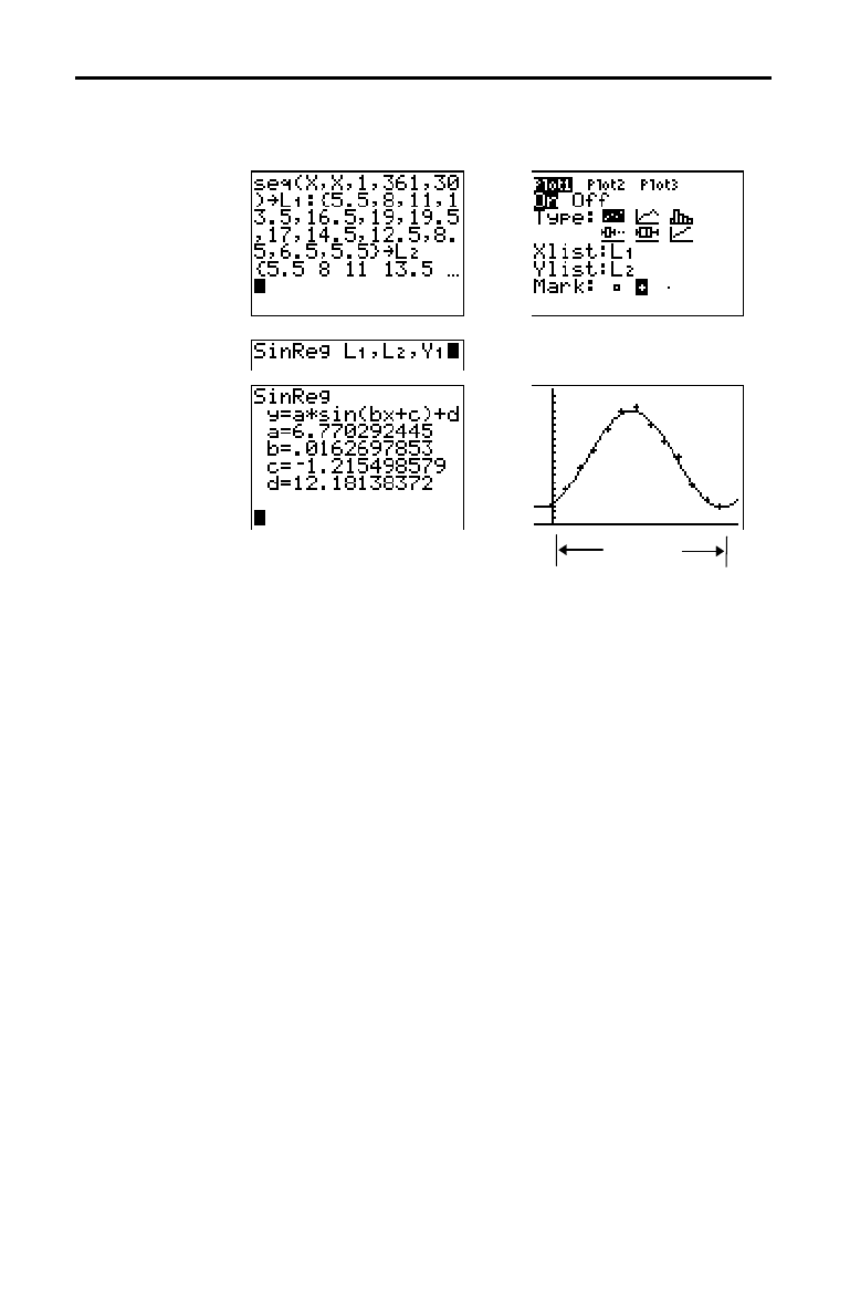
12-28 Statistics
8312STAT.DOC TI-83 international English Bob Fedorisko Revised: 02/19/01 12:42 PM Printed: 02/19/01 1:37
PM Page 28 of 38
Compute the regression model for the number of hours of
daylight in Alaska during one year.
&
&
With noisy data, you will achieve better convergence
results when you specify an accurate estimate for
period
.
You can obtain a
period
guess in either of two ways.
•
Plot the data and trace to determine the x-distance
between the beginning and end of one complete period,
or cycle. The illustration above and to the right
graphically depicts a complete period, or cycle.
•
Plot the data and trace to determine the x-distance
between the beginning and end of N complete periods,
or cycles. Then divide the total distance by N.
After your first attempt to use
SinReg and the default value
for
iterations
to fit the data, you may find the fit to be
approximately correct, but not optimal. For an optimal fit,
execute
SinReg 16,
Xlistname
,
Ylistname
,2
p
/
b
where
b
is
the value obtained from the previous
SinReg execution.
SinReg Example:
Daylight Hours in
Alaska for One
Year
1 period

Statistics 12-29
8312STAT.DOC TI-83 international English Bob Fedorisko Revised: 02/19/01 12:42 PM Printed: 02/19/01 1:37
PM Page 29 of 38
The statistical variables are calculated and stored as indicated below. To
access these variables for use in expressions, press
, and select
5:Statistics. Then select the
VARS
menu shown in the column below under
VARS
menu. If you edit a list or change the type of analysis, all statistical
variables are cleared.
Variables
1
.
Var
Stats
2
.
Var
Stats
Other
VARS
menu
mean of x values
vv
XY
sum of x values
G
x
G
x
G
sum of x
2
values
G
x
2
G
x
2
G
sample standard deviation of xSxSx
XY
population standard deviation of x
s
x
s
x
XY
number of data points nn
XY
mean of y values
w
XY
sum of y values
G
y
G
sum of y
2
values
G
y
2
G
sample standard deviation of ySy
XY
population standard deviation of y
s
y
XY
sum of x
…
y
G
xy
G
minimum of x values minX minX
XY
maximum of x values maxX maxX
XY
minimum of y values minY
XY
maximum of y values maxY
XY
1st quartile Q
1
PTS
median Med
PTS
3rd quartile Q
3
PTS
regression/fit coefficients a, b
EQ
polynomial, Logistic, and SinReg
coefficients
a, b, c,
d, e
EQ
correlation coefficient r
EQ
coefficient of determination r
2
, R
2
EQ
regression equation RegEQ
EQ
summary points (Med
.
Med only) x1, y1, x2,
y2, x3, y3
PTS
The first quartile (Q
1
) is the median of points between
minX and Med (median). The third quartile (Q
3
) is the
median of points between
Med and maxX.
Statistical Variables
Q
1
and Q
3
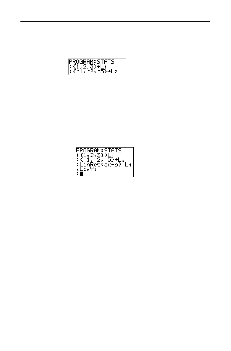
12-30 Statistics
8312STAT.DOC TI-83 international English Bob Fedorisko Revised: 02/19/01 12:42 PM Printed: 02/19/01 1:37
PM Page 30 of 38
You can enter statistical data, calculate statistical results,
and fit models to data from a program. You can enter
statistical data into lists directly within the program
(Chapter 11).
To perform a statistical calculation from a program, follow
these steps.
1. On a blank line in the program editor, select the type of
calculation from the
STAT CALC
menu.
2. Enter the names of the lists to use in the calculation.
Separate the list names with a comma.
3. Enter a comma and then the name of a
Y=
variable, if you
want to store the regression equation to a
Y=
variable.
Statistical Analysis in a Program
Entering Stat
Data
Statistical
Calculations
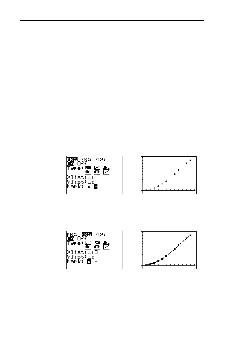
Statistics 12-31
8312STAT.DOC TI-83 international English Bob Fedorisko Revised: 02/19/01 12:42 PM Printed: 02/19/01 1:37
PM Page 31 of 38
You can plot statistical data that is stored in lists. The six
types of plots available are scatter plot, xyLine, histogram,
modified box plot, regular box plot, and normal probability
plot. You can define up to three plots.
To plot statistical data in lists, follow these steps.
1. Store the stat data in one or more lists.
2. Select or deselect
Y=
functions as appropriate.
3. Define the stat plot.
4. Turn on the plots you want to display.
5. Define the viewing window.
6. Display and explore the graph.
Scatter plots plot the data points from Xlist and Ylist as
coordinate pairs, showing each point as a box (
›
), cross
(
+ ), or dot (
¦
). Xlist and Ylist must be the same length.
You can use the same list for
Xlist and Ylist.
xyLine is a scatter plot in which the data points are plotted
and connected in order of appearance in
Xlist and Ylist.
You may want to use
SortA( or SortD( to sort the lists
before you plot them (page 12
.
20).
Statistical Plotting
Steps for Plotting
Statistical Data in
Lists
"
(Scatter)
Ó
(xyLine)
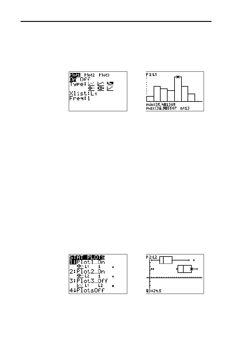
12-32 Statistics
8312STAT.DOC TI-83 international English Bob Fedorisko Revised: 02/19/01 12:42 PM Printed: 02/19/01 1:37
PM Page 32 of 38
Histogram plots one-variable data. The Xscl window variable
value determines the width of each bar, beginning at
Xmin.
ZoomStat adjusts Xmin, Xmax, Ymin, and Ymax to include all
values, and also adjusts
Xscl. The inequality
(
Xmax
N
Xmin)
à
Xscl
47 must be true. A value that occurs
on the edge of a bar is counted in the bar to the right.
ModBoxplot (modified box plot) plots one-variable data,
like the regular box plot, except points that are 1.5
ä
Interquartile Range beyond the quartiles. (The Interquartile
Range is defined as the difference between the third
quartile
Q
3
and the first quartile Q
1
.) These points are
plotted individually beyond the whisker, using the
Mark
(
›
or +
or
¦
) you select. You can trace these points, which
are called outliers.
The prompt for outlier points is
x=, except when the outlier
is the maximum point (
maxX) or the minimum point
(
minX). When outliers exist, the end of each whisker will
display
x=. When no outliers exist, minX and maxX are the
prompts for the end of each whisker.
Q
1
, Med (median),
and
Q
3
define the box (page 12
.
29).
Box plots are plotted with respect to
Xmin and Xmax, but
ignore
Ymin and Ymax. When two box plots are plotted, the
first one plots at the top of the screen and the second plots
in the middle. When three are plotted, the first one plots at
the top, the second in the middle, and the third at the
bottom.
Ò
(Histogram)
Õ
(ModBoxplot)
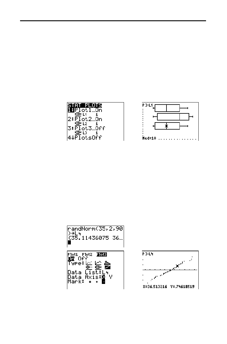
Statistics 12-33
8312STAT.DOC TI-83 international English Bob Fedorisko Revised: 02/19/01 12:42 PM Printed: 02/19/01 1:37
PM Page 33 of 38
Boxplot (regular box plot) plots one-variable data. The
whiskers on the plot extend from the minimum data point
in the set (
minX) to the first quartile (Q
1
) and from the third
quartile (
Q
3
) to the maximum point (maxX). The box is
defined by
Q
1
, Med (median), and Q
3
(page 12
.
29).
Box plots are plotted with respect to
Xmin and Xmax, but
ignore
Ymin and Ymax. When two box plots are plotted, the
first one plots at the top of the screen and the second plots
in the middle. When three are plotted, the first one plots at
the top, the second in the middle, and the third at the
bottom.
NormProbPlot (normal probability plot) plots each
observation
X in Data List versus the corresponding
quantile
z of the standard normal distribution. If the plotted
points lie close to a straight line, then the plot indicates
that the data are normal.
Enter a valid list name in the
Data List field. Select X or Y
for the Data Axis setting.
•
If you select
X, the TI
-
83 plots the data on the x-axis and
the z-values on the y-axis.
•
If you select
Y, the TI
-
83 plots the data on the y-axis and
the z-values on the x-axis.
Ö
(Boxplot)
Ô
(NormProbPlot)
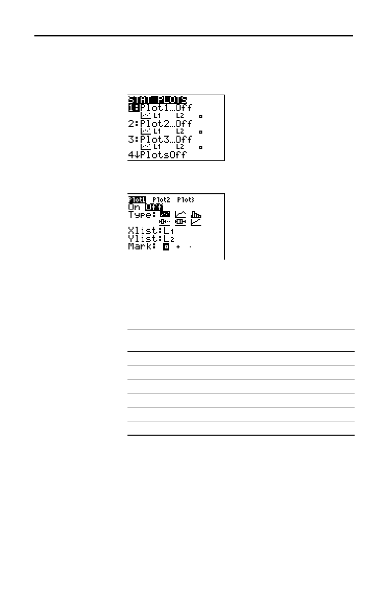
12-34 Statistics
8312STAT.DOC TI-83 international English Bob Fedorisko Revised: 02/19/01 12:42 PM Printed: 02/19/01 1:37
PM Page 34 of 38
To define a plot, follow these steps.
1. Press
y
[
STAT PLOT
]. The
STAT PLOTS
menu is
displayed with the current plot definitions.
2. Select the plot you want to use. The stat plot editor is
displayed for the plot you selected.
3. Press
Í
to select On if you want to plot the
statistical data immediately. The definition is stored
whether you select
On or Off.
4. Select the type of plot. Each type prompts for the
options checked in this table.
Plot Type
XList YList Mark Freq
Data
List
Data
Axis
"
Scatter
œœœ
Ó
xyLine
œœœ
Ò
Histogram
œœœœ
Õ
ModBoxplot
œœœ
Ö
Boxplot
œœœœ
Ô
NormProbPlot
œœœ
5. Enter list names or select options for the plot type.
•
Xlist (list name containing independent data)
•
Ylist (list name containing dependent data)
•
Mark (
›
or + or
¦
)
•
Freq (frequency list for Xlist elements; default is 1)
•
Data List (list name for NormProbPlot)
•
Data Axis (axis on which to plot Data List)
Defining the
Plots
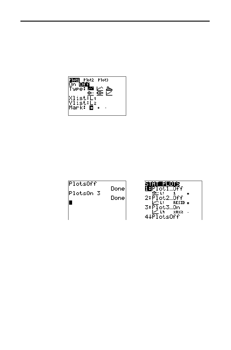
Statistics 12-35
8312STAT.DOC TI-83 international English Bob Fedorisko Revised: 02/19/01 12:42 PM Printed: 02/19/01 1:37
PM Page 35 of 38
Each stat plot has a unique stat plot editor. The name of
the current stat plot (
Plot1, Plot2, or Plot3) is highlighted in
the top line of the stat plot editor. To display the stat plot
editor for a different plot, press
}
,
~
, and
|
to move the
cursor onto the name in the top line, and then press
Í
.
The stat plot editor for the selected plot is displayed, and
the selected name remains highlighted.
PlotsOn and PlotsOff allow you to turn on or turn off stat
plots from the home screen or a program. With no plot
number,
PlotsOn turns on all plots and PlotsOff turns off all
plots. With one or more plot numbers (
1, 2, and 3), PlotsOn
turns on specified plots, and PlotsOff turns off specified
plots.
PlotsOff [1,2,3]
PlotsOn [1,2,3]
Note:
You also can turn on and turn off stat plots in the top line of the
Y= editor (Chapter 3).
Displaying Other
Stat Plot Editors
Turning On and
Turning Off Stat
Plots

12-36 Statistics
8312STAT.DOC TI-83 international English Bob Fedorisko Revised: 02/19/01 12:42 PM Printed: 02/19/01 1:37
PM Page 36 of 38
Stat plots are displayed on the current graph. To define the
viewing window, press
p
and enter values for the
window variables.
ZoomStat redefines the viewing window
to display all statistical data points.
When you trace a scatter plot or xyLine, tracing begins at
the first element in the lists.
When you trace a histogram, the cursor moves from the
top center of one column to the top center of the next,
starting at the first column.
When you trace a box plot, tracing begins at
Med (the
median). Press
|
to trace to
Q
1
and minX. Press
~
to trace
to
Q
3
and maxX.
When you press
}
or
†
to move to another plot or to
another
Y=
function, tracing moves to the current or
beginning point on that plot (not the nearest pixel).
The
ExprOn/ExprOff format setting applies to stat plots
(Chapter 3).When
ExprOn is selected, the plot number and
plotted data lists are displayed in the top-left corner.
Defining the
Viewing Window
Tracing a Stat
Plot
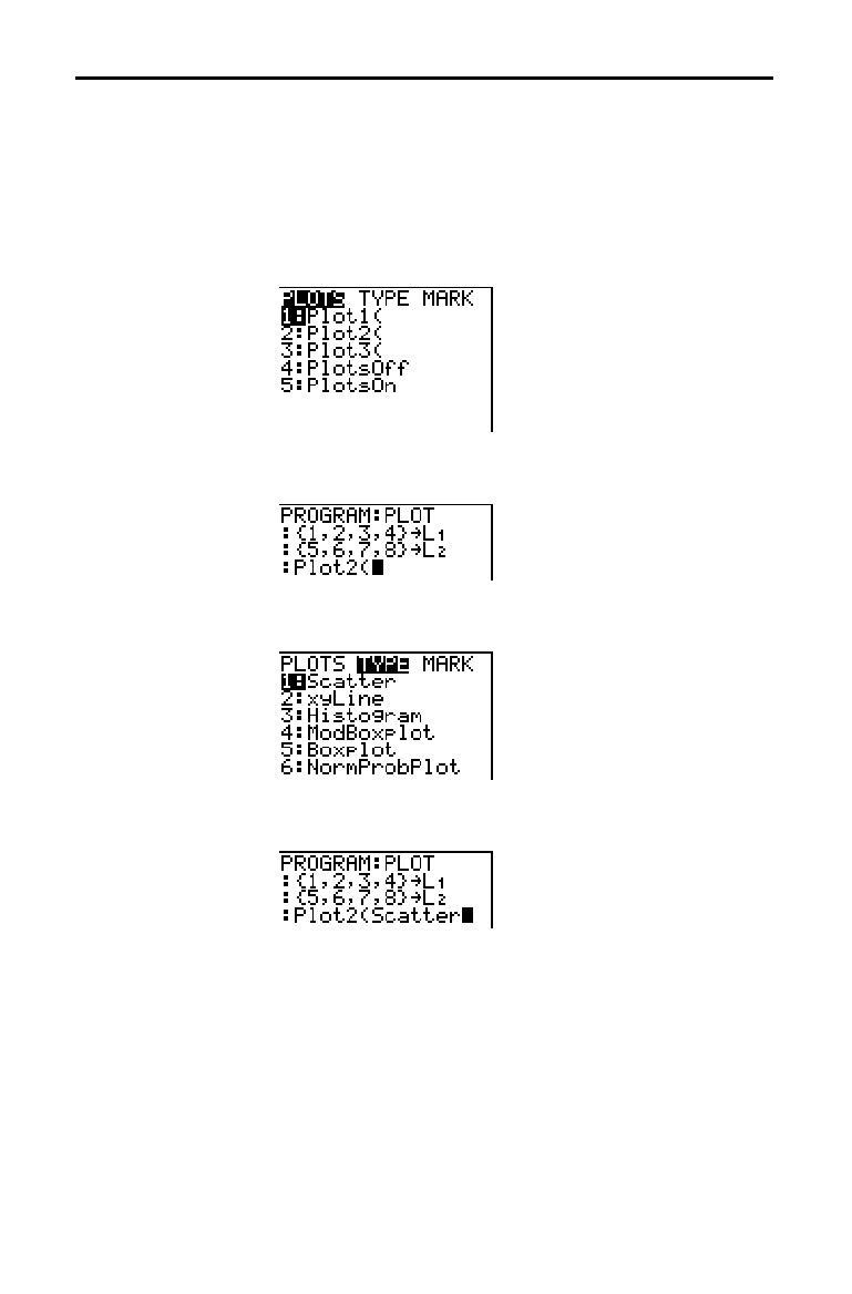
Statistics 12-37
8312STAT.DOC TI-83 international English Bob Fedorisko Revised: 02/19/01 12:42 PM Printed: 02/19/01 1:37
PM Page 37 of 38
To display a stat plot from a program, define the plot, and
then display the graph.
To define a stat plot from a program, begin on a blank line
in the program editor and enter data into one or more lists;
then, follow these steps.
1. Press
y
[
STAT PLOT
] to display the
STAT PLOTS
menu.
2. Select the plot to define, which pastes Plot1(, Plot2(, or
Plot3( to the cursor location.
3. Press
y
[
STAT PLOT
]
~
to display the
STAT TYPE
menu.
4. Select the type of plot, which pastes the name of the
plot type to the cursor location.
Statistical Plotting in a Program
Defining a Stat
Plot in a Program
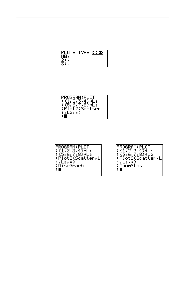
12-38 Statistics
8312STAT.DOC TI-83 international English Bob Fedorisko Revised: 02/19/01 12:42 PM Printed: 02/19/01 1:37
PM Page 38 of 38
5. Press
¢
. Enter the list names, separated by commas.
6. Press
¢
y
[
STAT PLOT
]
|
to display the
STAT PLOT MARK
menu. (This step is not necessary if
you selected
3:Histogram or 5:Boxplot in step 4.)
Select the type of mark (
›
or + or
¦
) for each data point.
The selected mark symbol is pasted to the cursor
location.
7. Press
¤
Í
to complete the command line.
To display a plot from a program, use the DispGraph
instruction (Chapter 16) or any of the
ZOOM
instructions
(Chapter 3).
Displaying a Stat
Plot from a
Program

Inferential Statistics and Distributions 13-1
8313INFE.DOC TI-83 international English Bob Fedorisko Revised: 02/19/01 12:47 PM Printed: 02/19/01 1:38 PM
Page 1 of 36
13
Inferential Statistics
and Distributions
Getting Started: Mean Height of a Population
............
13-2
Inferential Stat Editors
...................................
13-6
STAT TESTS
Menu
......................................
13-9
Inferential Statistics Input Descriptions
..................
13-26
Test and Interval Output Variables
.......................
13-28
Distribution Functions
...................................
13-29
Distribution Shading
.....................................
13-35
Contents
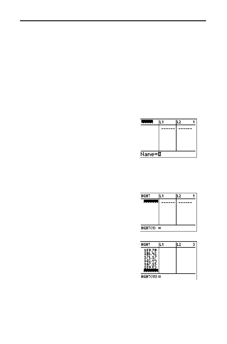
13-2 Inferential Statistics and Distributions
8313INFE.DOC TI-83 international English Bob Fedorisko Revised: 02/19/01 12:47 PM Printed: 02/19/01 1:38 PM
Page 2 of 36
Getting Started is a fast-paced introduction. Read the chapter for details.
Suppose you want to estimate the mean height of a population of women given
the random sample below. Because heights among a biological population tend
to be normally distributed, a
t
distribution confidence interval can be used
when estimating the mean. The 10 height values below are the first 10 of 90
values, randomly generated from a normally distributed population with an
assumed mean of 165.1 cm. and a standard deviation of 6.35 cm.
(
randNorm(165.1,6.35,90) with a seed of 789).
Height (in cm.) of Each of 10 Women
169.43 168.33 159.55 169.97 159.79 181.42 171.17 162.04 167.15 159.53
1. Press
…
Í
to display the stat list
editor.
Press
}
to move the cursor onto
L
1
, and
then press
y
[
INS
]. The Name= prompt is
displayed on the bottom line. The
Ø
cursor
indicates that alpha-lock is on. The
existing list name columns shift to the
right.
Note:
Your stat editor may not look like the one
pictured here, depending on the lists you have
already stored.
2. Enter [
H
] [
G
] [
H
] [
T
] at the Name= prompt,
and then press
Í
. The list to which
you will store the women’s height data is
created.
Press
†
to move the cursor onto the first
row of the list.
HGHT(1)=
is displayed on the
bottom line.
3. Press 169
Ë
43 to enter the first height
value. As you enter it, it is displayed on the
bottom line.
Press
Í
. The value is displayed in the
first row, and the rectangular cursor
moves to the next row.
Enter the other nine height values the
same way.
Getting Started: Mean Height of a Population
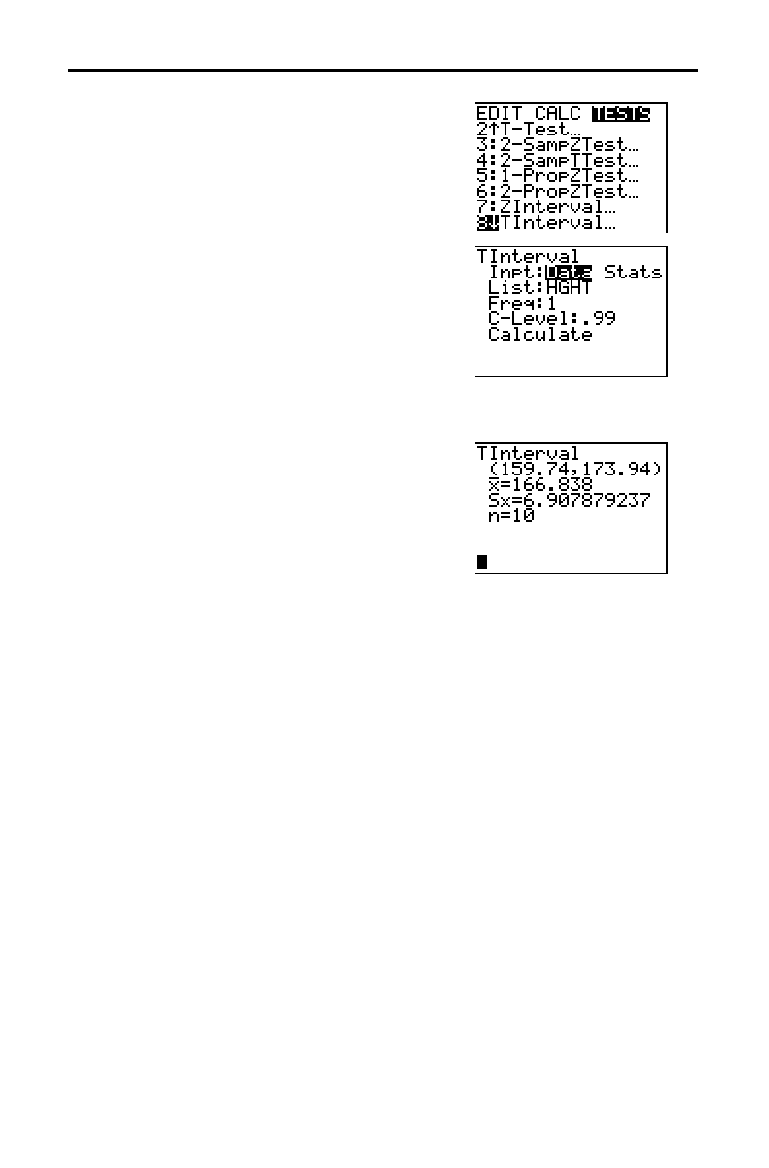
Inferential Statistics and Distributions 13-3
8313INFE.DOC TI-83 international English Bob Fedorisko Revised: 02/19/01 12:47 PM Printed: 02/19/01 1:38 PM
Page 3 of 36
4. Press
…
|
to display the
STAT TESTS
menu, and then press
†
until 8:TInterval is
highlighted.
5. Press
Í
to select 8:TInterval. The
inferential stat editor for
TInterval is
displayed. If
Data is not selected for Inpt:,
press
|
Í
to select
Data.
Press
†
and [
H
] [
G
] [
H
] [
T
] at the List:
prompt (alpha-lock is on).
Press
†
†
Ë
99 to enter a 99 percent
confidence level at the
C
.
Level: prompt.
6. Press
†
to move the cursor onto Calculate,
and then press
Í
. The confidence
interval is calculated, and the
TInterval
results are displayed on the home screen.
Interpret the results.
The first line,
(159.74,173.94), shows that the 99 percent confidence interval for
the population mean is between about 159.74 cm. and 173.94 cm. This is about
a 14.2 cm. spread.
The .99 confidence level indicates that in a very large number of samples, we
expect 99 percent of the intervals calculated to contain the population mean.
The actual mean of the population sampled is 165.1 cm. (introduction; page
13
.
2), which is in the calculated interval.
The second line gives the mean height of the sample
þ
used to compute this
interval. The third line gives the sample standard deviation
Sx. The bottom line
gives the sample size
n.
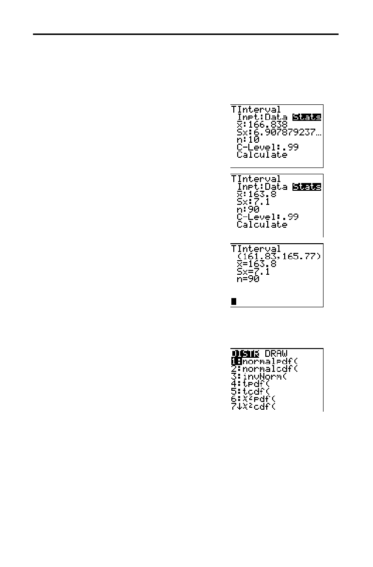
13-4 Inferential Statistics and Distributions
8313INFE.DOC TI-83 international English Bob Fedorisko Revised: 02/19/01 12:47 PM Printed: 02/19/01 1:38 PM
Page 4 of 36
To obtain a more precise bound on the population mean
m
of women’s heights,
increase the sample size to 90. Use a sample mean
þ
of 163.8 and sample
standard deviation
Sx of 7.1 calculated from the larger random sample
(introduction; page 13
.
2). This time, use the
Stats (summary statistics) input
option.
7. Press
…
|
8 to display the inferential
stat editor for
TInterval.
Press
~
Í
to select
Inpt:Stats. The
editor changes so that you can enter
summary statistics as input.
8. Press
†
163
Ë
8
Í
to store 163.8 to
þ
.
Press
7
Ë
1
Í
to store 7.1 to Sx.
Press
90
Í
to store 90 to n.
9. Press
†
to move the cursor onto Calculate,
and then press
Í
to calculate the new
99 percent confidence interval. The results
are displayed on the home screen.
If the height distribution among a population of women is normally distributed
with a mean
m
of 165.1 cm. and a standard deviation
σ
of 6.35 cm., what height
is exceeded by only 5 percent of the women (the 95th percentile)?
10. Press
‘
to clear the home screen.
Press
y
[
DISTR
] to display the
DISTR
(distributions) menu.
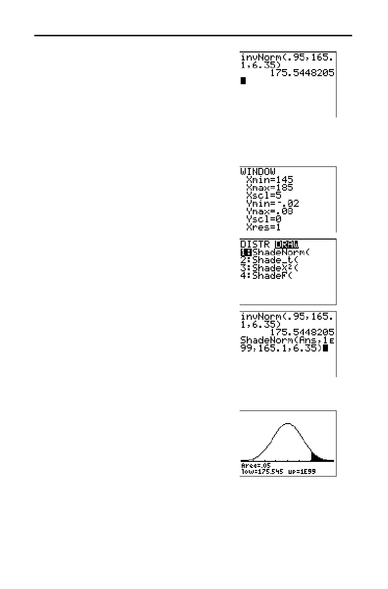
Inferential Statistics and Distributions 13-5
8313INFE.DOC TI-83 international English Bob Fedorisko Revised: 02/19/01 12:47 PM Printed: 02/19/01 1:38 PM
Page 5 of 36
11. Press 3 to paste invNorm( to the home
screen.
Press
Ë
95
¢
165
Ë
1
¢
6
Ë
35
¤
Í
.
.95 is the area, 165.1 is
µ
, and 6.35 is
σ
.
The result is displayed on the home screen; it shows that five percent of the
women are taller than 175.5 cm.
Now graph and shade the top 5 percent of the population.
12. Press
p
and set the window
variables to these values.
Xmin=145 Ymin=
L
.02 Xres=1
Xmax=185 Ymax=.08
Xscl=5 Yscl=0
13. Press
y
[
DISTR
]
~
to display the
DISTR
DRAW
menu.
14. Press
Í
to paste ShadeNorm( to the
home screen.
Press
y
[
ANS
]
¢
1
y
[
EE
] 99
¢
165
Ë
1
¢
6
Ë
35
¤
.
Ans (175.5448205 from step 11) is the
lower bound. 1
å
99 is the upper bound. The
normal curve is defined by a mean
µ
of
165.1 and a standard deviation
σ
of 6.35.
15. Press
Í
to plot and shade the normal
curve.
Area is the area above the 95th percentile.
low is the lower bound. up is the upper
bound.
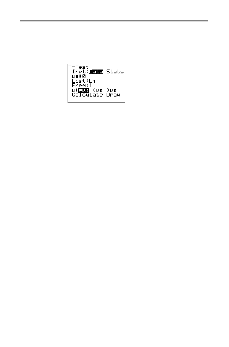
13-6 Inferential Statistics and Distributions
8313INFE.DOC TI-83 international English Bob Fedorisko Revised: 02/19/01 12:47 PM Printed: 02/19/01 1:38 PM
Page 6 of 36
When you select a hypothesis test or confidence interval
instruction from the home screen, the appropriate
inferential statistics editor is displayed. The editors vary
according to each test or interval’s input requirements.
Below is the inferential stat editor for
T
.
Test.
Note:
When you select the
ANOVA(
instruction, it is pasted to the
home screen.
ANOVA(
does not have an editor screen.
To use an inferential stat editor, follow these steps.
1. Select a hypothesis test or confidence interval from the
STAT TESTS
menu. The appropriate editor is displayed.
2. Select
Data or Stats input, if the selection is available.
The appropriate editor is displayed.
3. Enter real numbers, list names, or expressions for each
argument in the editor.
4. Select the alternative hypothesis (
ƒ
, <, or >) against
which to test, if the selection is available.
5. Select
No or Yes for the Pooled option, if the selection is
available.
6. Select
Calculate or Draw (when Draw is available) to
execute the instruction.
•
When you select
Calculate, the results are displayed
on the home screen.
•
When you select
Draw, the results are displayed in a
graph.
This chapter describes the selections in the above steps for
each hypothesis test and confidence interval instruction.
Inferential Stat Editors
Displaying the
Inferential Stat
Editors
Using an
Inferential Stat
Editor
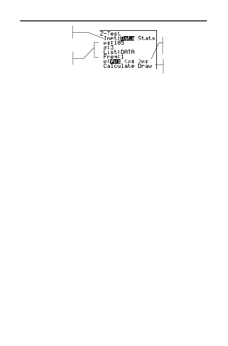
Inferential Statistics and Distributions 13-7
8313INFE.DOC TI-83 international English Bob Fedorisko Revised: 02/19/01 12:47 PM Printed: 02/19/01 1:38 PM
Page 7 of 36
Most inferential stat editors prompt you to select one of
two types of input. (
1
.
PropZInt and 2
.
PropZTest, 1
.
PropZInt
and 2
.
PropZInt,
c
2
.
Test
, and LinRegTTest do not.)
•
Select
Data to enter the data lists as input.
•
Select
Stats to enter summary statistics, such as
þ
, Sx,
and n, as input.
To select
Data or Stats, move the cursor to either Data or
Stats, and then press
Í
.
Inferential stat editors require a value for every argument.
If you do not know what a particular argument symbol
represents, see the tables on pages 13
.
26 and 13
.
27.
When you enter values in any inferential stat editor, the
TI
.
83 stores them in memory so that you can run many
tests or intervals without having to reenter every value.
Most of the inferential stat editors for the hypothesis tests
prompt you to select one of three alternative hypotheses.
•
The first is a
ƒ
alternative hypothesis, such as
mƒm
0
for
the Z
.
Test.
•
The second is a
< alternative hypothesis, such as
m
1<
m
2
for the 2
.
SampTTest.
•
The third is a
> alternative hypothesis, such as p1>p2 for
the 2
.
PropZTest.
To select an alternative hypothesis, move the cursor to the
appropriate alternative, and then press
Í
.
Selecting Data or
Stats
Entering the
Values for
Arguments
Selecting an
Alternative
Hypothesis
(
ƒ
< >)
Enter values for
arguments
Select an alternative
hypothesis
Select
Calculate
or
Draw
output
Select
Data
or
Stats
input

13-8 Inferential Statistics and Distributions
8313INFE.DOC TI-83 international English Bob Fedorisko Revised: 02/19/01 12:47 PM Printed: 02/19/01 1:38 PM
Page 8 of 36
Pooled (2
.
SampTTest and 2
.
SampTInt only) specifies
whether the variances are to be pooled for the calculation.
•
Select
No if you do not want the variances pooled.
Population variances can be unequal.
•
Select
Yes if you want the variances pooled. Population
variances are assumed to be equal.
To select the
Pooled option, move the cursor to Yes, and
then press
Í
.
After you have entered all arguments in an inferential stat
editor for a hypothesis test, you must select whether you
want to see the calculated results on the home screen
(
Calculate) or on the graph screen (Draw).
•
Calculate calculates the test results and displays the
outputs on the home screen.
•
Draw draws a graph of the test results and displays the
test statistic and p-value with the graph. The window
variables are adjusted automatically to fit the graph.
To select
Calculate or Draw, move the cursor to either
Calculate or Draw, and then press
Í
. The instruction is
immediately executed.
After you have entered all arguments in an inferential stat
editor for a confidence interval, select
Calculate to display
the results. The
Draw option is not available.
When you press
Í
,
Calculate calculates the confidence
interval results and displays the outputs on the home
screen.
To paste a hypothesis test or confidence interval
instruction to the home screen without displaying the
corresponding inferential stat editor, select the instruction
you want from the
CATALOG
menu. Appendix A describes
the input syntax for each hypothesis test and confidence
interval instruction.
Note:
You can paste a hypothesis test or confidence interval
instruction to a command line in a program. From within the program
editor, select the instruction from either the
CATALOG
(Chapter 15)
or the
STAT TESTS
menu.
Selecting the
Pooled Option
Selecting
Calculate or Draw
for a Hypothesis
Test
Selecting
Calculate for a
Confidence
Interval
Bypassing the
Inferential Stat
Editors

Inferential Statistics and Distributions 13-9
8313INFE.DOC TI-83 international English Bob Fedorisko Revised: 02/19/01 12:47 PM Printed: 02/19/01 1:38 PM
Page 9 of 36
To display the
STAT TESTS
menu, press
…
|
. When you
select an inferential statistics instruction, the appropriate
inferential stat editor is displayed.
Most
STAT TESTS
instructions store some output variables
to memory. Most of these output variables are in the
TEST
secondary menu (
VARS
menu; 5:Statistics). For a list of
these variables, see page 13
.
28.
EDIT CALC TESTS
1: Z-Test...
Test for 1
m
, known
s
2: T-Test...
Test for 1
m
, unknown
s
3: 2-SampZTest...
Test comparing 2
m
’s, known
s
’s
4: 2-SampTTest...
Test comparing 2
m
’s, unknown
s
’s
5: 1-PropZTest...
Test for 1 proportion
6: 2-PropZTest...
Test comparing 2 proportions
7: ZInterval...
Confidence interval for 1
m
, known
s
8: TInterval...
Confidence interval for 1
m
, unknown
s
9: 2-SampZInt...
Conf. int. for diff. of 2
m
’s, known
s
’s
0: 2-SampTInt...
Conf. int. for diff. of 2
m
’s, unknown
s
’s
A: 1-PropZInt...
Confidence int. for 1 proportion
B: 2-PropZInt...
Confidence int. for diff. of 2 props
C:
c
2-Test...
Chi-square test for 2-way tables
D: 2-Samp
Û
Test...
Test comparing 2
s
’s
E: LinRegTTest...
t
test for regression slope and
r
F: ANOVA(
One-way analysis of variance
Note:
When a new test or interval is computed, all previous output
variables are invalidated.
In this chapter, the description of each
STAT TESTS
instruction shows the unique inferential stat editor for that
instruction with example arguments.
•
Descriptions of instructions that offer the
Data/Stats
input choice show both types of input screens.
•
Descriptions of instructions that do not offer the
Data/Stats input choice show only one input screen.
The description then shows the unique output screen for
that instruction with the example results.
•
Descriptions of instructions that offer the
Calculate/Draw output choice show both types of
screens: calculated and graphic results.
•
Descriptions of instructions that offer only the
Calculate
output choice show the calculated results on the home
screen.
STAT TESTS Menu
STAT TESTS
Menu
Inferential Stat
Editors for the
STAT TESTS
Instructions
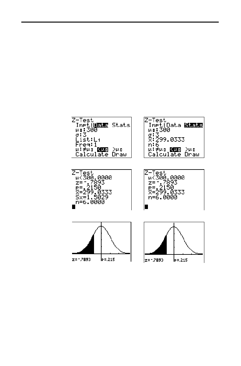
13-10 Inferential Statistics and Distributions
8313INFE.DOC TI-83 international English Bob Fedorisko Revised: 02/19/01 12:47 PM Printed: 02/19/01 1:38 PM
Page 10 of 36
Z
.
Test (one-sample
z
test; item 1) performs a hypothesis
test for a single unknown population mean
m
when the
population standard deviation
s
is known. It tests the null
hypothesis H
0
:
m
=
m
0
against one of the alternatives below.
•
H
a
:
mƒm
0
(
m
:
ƒm
0
)
•
H
a
:
m
<
m
0
(
m
:<
m
0
)
•
H
a
:
m
>
m
0
(
m
:>
m
0
)
In the example:
L
1
={299.4 297.7 301 298.9 300.2 297}
Data Stats
Input:
,,
Calculated results:
,,
Drawn results:
Note:
All examples on pages13
.
10 through 13
.
25 assume a fixed-
decimal mode setting of
4
(Chapter 1). If you set the decimal mode to
Float
or a different fixed-decimal setting, your output may differ from
the output in the examples.
Z
.
Test
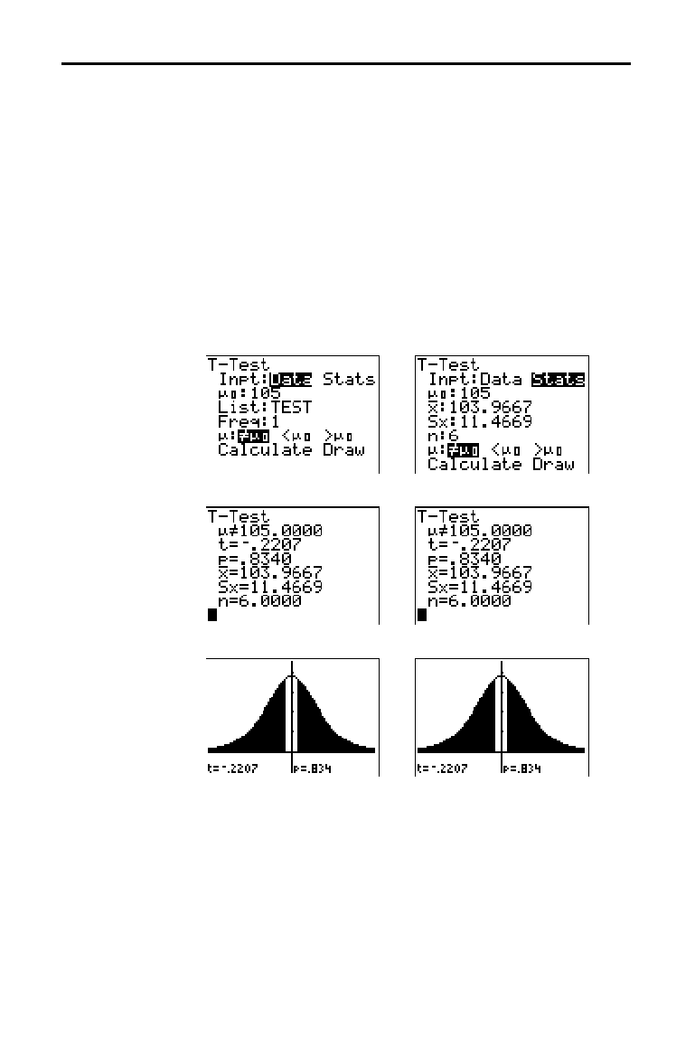
Inferential Statistics and Distributions 13-11
8313INFE.DOC TI-83 international English Bob Fedorisko Revised: 02/19/01 12:47 PM Printed: 02/19/01 1:38 PM
Page 11 of 36
T
.
Test (one-sample
t
test; item 2) performs a hypothesis
test for a single unknown population mean
m
when the
population standard deviation
s
is unknown. It tests the
null hypothesis H
0
:
m
=
m
0
against one of the alternatives
below.
•
H
a
:
mƒm
0
(
m
:
ƒm
0
)
•
H
a
:
m
<
m
0
(
m
:<
m
0
)
•
H
a
:
m
>
m
0
(
m
:>
m
0
)
In the example:
TEST={91.9 97.8 111.4 122.3 105.4 95}
Data Stats
Input:
,,
Calculated results:
,,
Drawn results:
T
.
Test
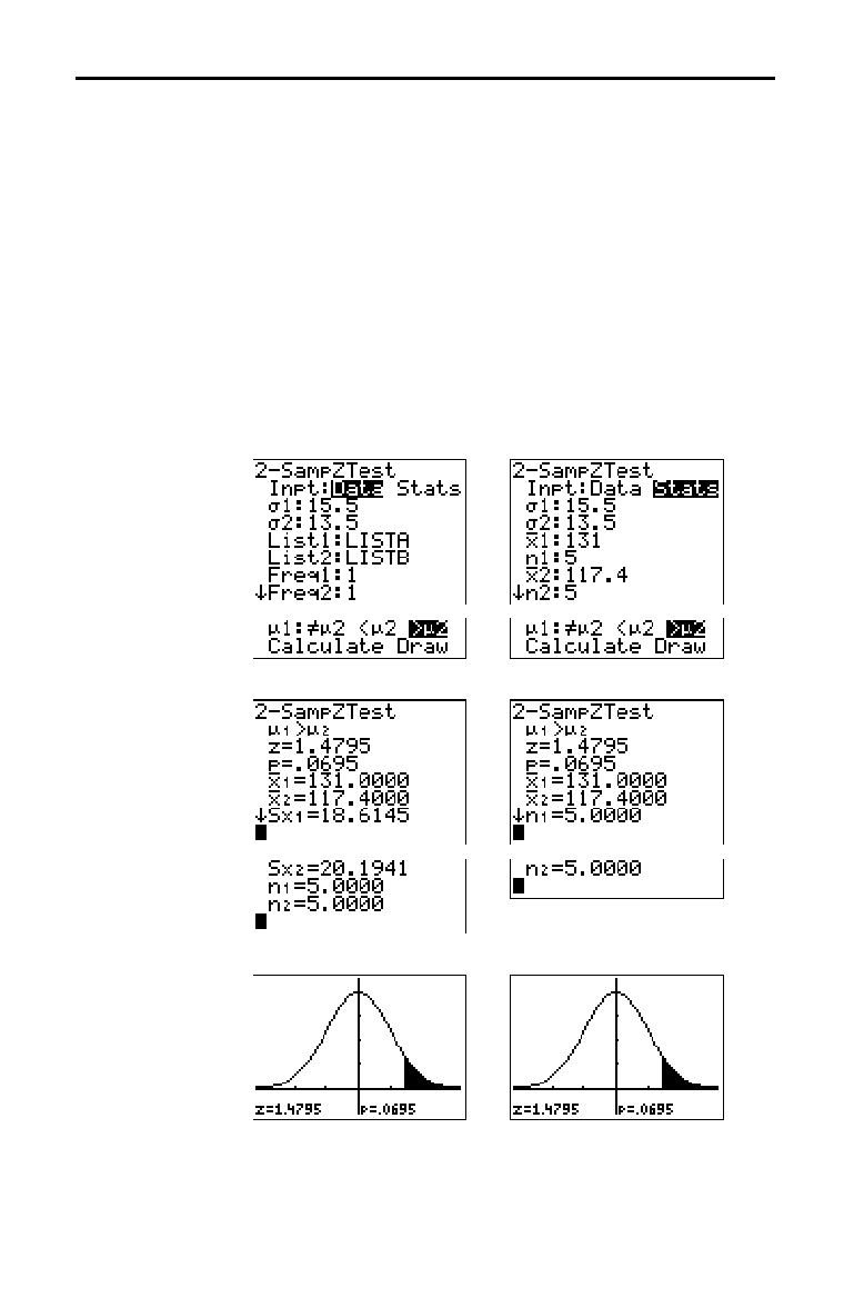
13-12 Inferential Statistics and Distributions
8313INFE.DOC TI-83 international English Bob Fedorisko Revised: 02/19/01 12:47 PM Printed: 02/19/01 1:38 PM
Page 12 of 36
2
.
SampZTest (two-sample
z
test; item 3) tests the equality
of the means of two populations (
m
1
and
m
2
) based on
independent samples when both population standard
deviations (
s
1
and
s
2
) are known. The null hypothesis
H
0
:
m
1
=
m
2
is tested against one of the alternatives below.
•
H
a
:
m
1
ƒm
2
(
m
1:
ƒm
2
)
•
H
a
:
m
1
<
m
2
(
m
1:<
m
2
)
•
H
a
:
m
1
>
m
2
(
m
1:>
m
2
)
In the example:
LISTA={154 109 137 115 140}
LISTB={108 115 126 92 146}
Data Stats
Input:
,,
Calculated results:
,,
Drawn results:
2
.
SampZTest
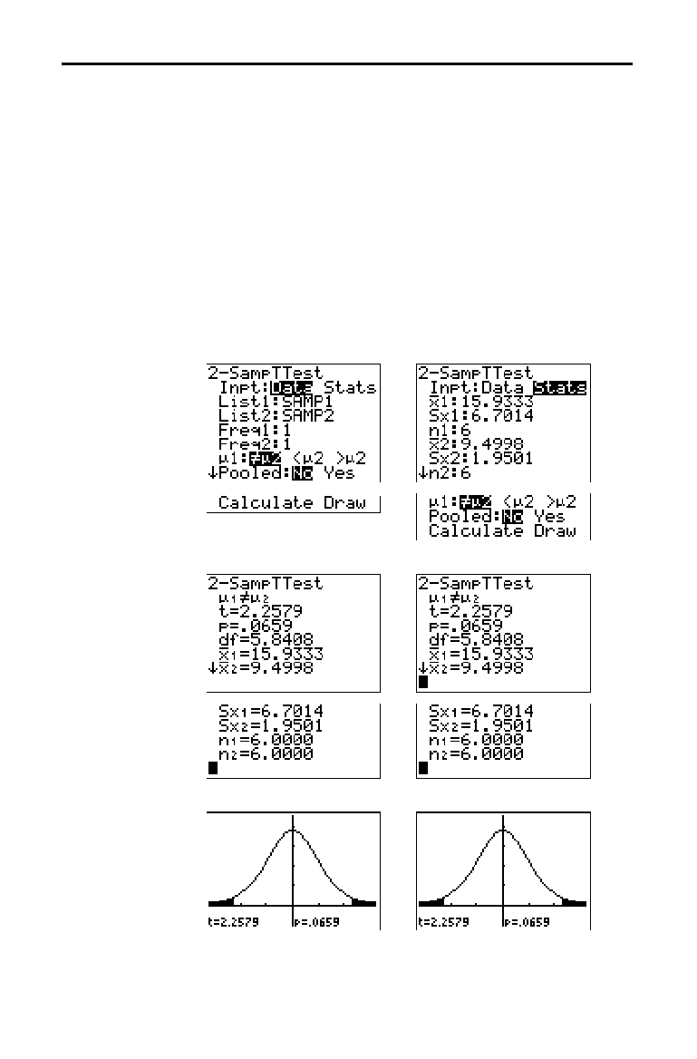
Inferential Statistics and Distributions 13-13
8313INFE.DOC TI-83 international English Bob Fedorisko Revised: 02/19/01 12:47 PM Printed: 02/19/01 1:38 PM
Page 13 of 36
2
.
SampTTest (two-sample
t
test; item 4) tests the equality
of the means of two populations (
m
1
and
m
2
) based on
independent samples when neither population standard
deviation (
s
1
or
s
2
) is known. The null hypothesis
H
0
:
m
1
=
m
2
is tested against one of the alternatives below.
•
H
a
:
m
1
ƒm
2
(
m
1:
ƒm
2
)
•
H
a
:
m
1
<
m
2
(
m
1:<
m
2
)
•
H
a
:
m
1
>
m
2
(
m
1:>
m
2
)
In the example:
SAMP1={12.207 16.869 25.05 22.429 8.456 10.589}
SAMP2={11.074 9.686 12.064 9.351 8.182 6.642}
Data Stats
Input:
,,
Calculated results:
,,
Drawn results:
2
.
SampTTest
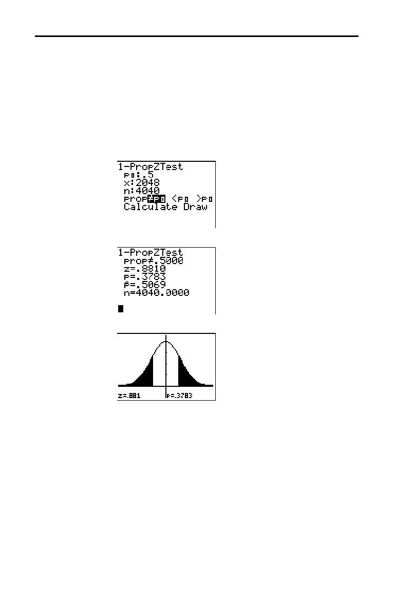
13-14 Inferential Statistics and Distributions
8313INFE.DOC TI-83 international English Bob Fedorisko Revised: 02/19/01 12:47 PM Printed: 02/19/01 1:38 PM
Page 14 of 36
1
.
PropZTest (one-proportion
z
test; item 5) computes a test
for an unknown proportion of successes
(prop). It takes as
input the count of successes in the sample
x
and the count
of observations in the sample
n
.
1
.
PropZTest tests the null
hypothesis H
0
: prop=p
0
against one of the alternatives
below.
•
H
a
: prop
ƒ
p
0
(prop:
ƒ
p
0
)
•
H
a
: prop<p
0
(prop:<p
0
)
•
H
a
: prop>p
0
(prop:>p
0
)
Input:
,
Calculated results:
,
Drawn results:
)
1-PropZTest
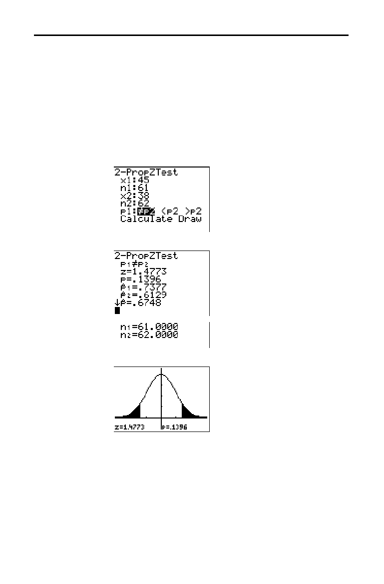
Inferential Statistics and Distributions 13-15
8313INFE.DOC TI-83 international English Bob Fedorisko Revised: 02/19/01 12:47 PM Printed: 02/19/01 1:38 PM
Page 15 of 36
2
.
PropZTest (two-proportion
z
test; item 6) computes a test
to compare the proportion of successes (p
1
and p
2
) from
two populations. It takes as input the count of successes in
each sample (
x
1
and
x
2
) and the count of observations in
each sample (
n
1
and
n
2
). 2
.
PropZTest tests the null
hypothesis H
0
: p
1
=p
2
(using the pooled sample proportion
Ç
) against one of the alternatives below.
•
H
a
: p
1
ƒ
p
2
(p1:
ƒ
p2)
•
H
a
: p
1
<p
2
(p1:<p2)
•
H
a
: p
1
>p
2
(p1:>p2)
Input:
,
Calculated results:
,
Drawn results:
2-PropZTest
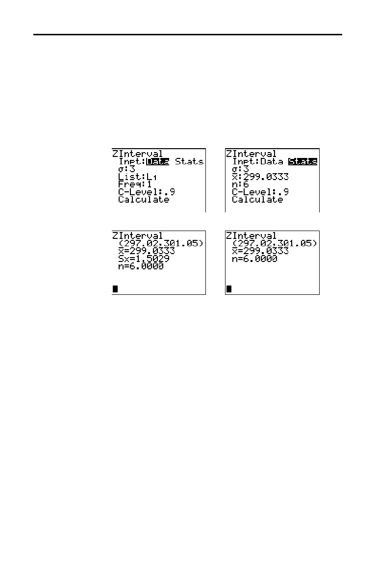
13-16 Inferential Statistics and Distributions
8313INFE.DOC TI-83 international English Bob Fedorisko Revised: 02/19/01 12:47 PM Printed: 02/19/01 1:38 PM
Page 16 of 36
ZInterval (one-sample
z
confidence interval; item 7)
computes a confidence interval for an unknown population
mean
m
when the population standard deviation
s
is
known. The computed confidence interval depends on the
user-specified confidence level.
In the example:
L
1
={299.4 297.7 301 298.9 300.2 297}
Data Stats
Input:
,,
Calculated results:
ZInterval
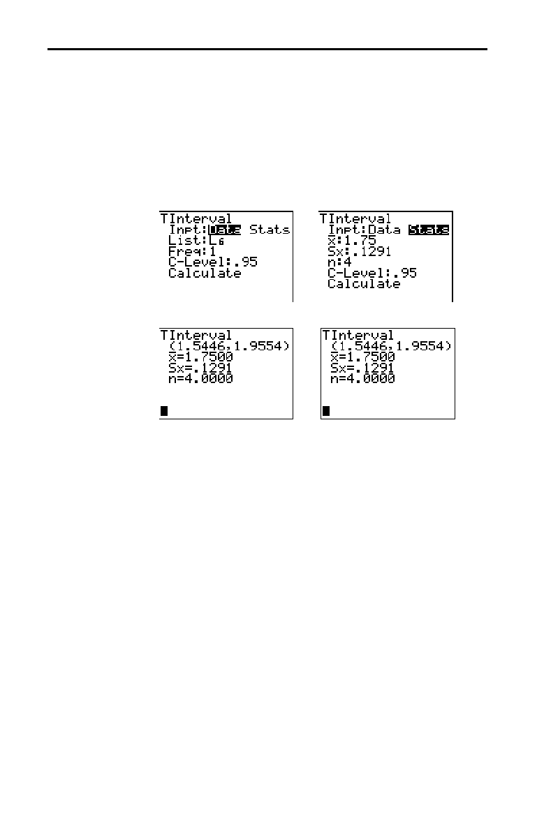
Inferential Statistics and Distributions 13-17
8313INFE.DOC TI-83 international English Bob Fedorisko Revised: 02/19/01 12:47 PM Printed: 02/19/01 1:38 PM
Page 17 of 36
TInterval (one-sample
t
confidence interval; item 8)
computes a confidence interval for an unknown population
mean
m
when the population standard deviation
s
is
unknown. The computed confidence interval depends on
the user-specified confidence level.
In the example:
L
6
={1.6 1.7 1.8 1.9}
Data Stats
Input:
,,
Calculated results:
TInterval
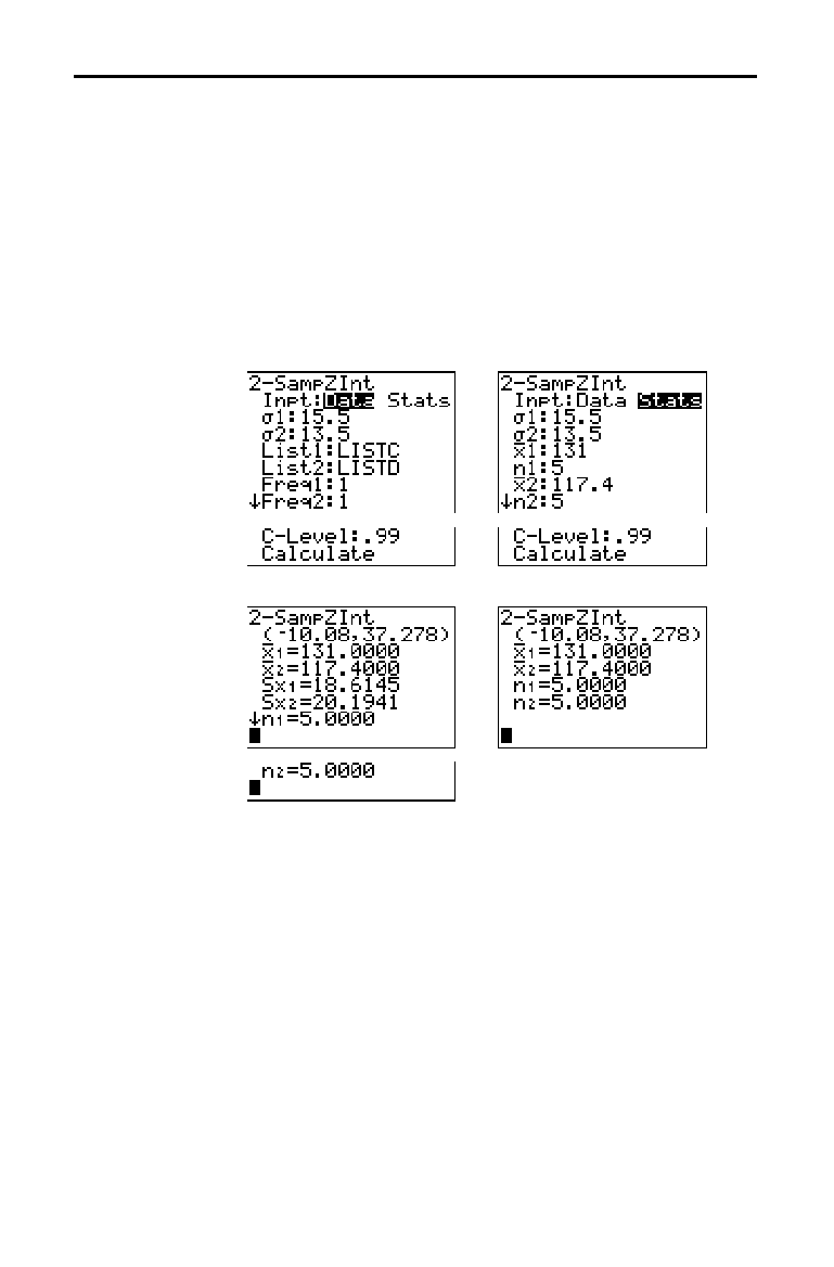
13-18 Inferential Statistics and Distributions
8313INFE.DOC TI-83 international English Bob Fedorisko Revised: 02/19/01 12:47 PM Printed: 02/19/01 1:38 PM
Page 18 of 36
2
.
SampZInt (two-sample
z
confidence interval; item 9)
computes a confidence interval for the difference between
two population means (
m
1
Nm
2
) when both population
standard deviations (
s
1
and
s
2
) are known. The computed
confidence interval depends on the user-specified
confidence level.
In the example:
LISTC={154 109 137 115 140}
LISTD={108 115 126 92 146}
Data Stats
Input:
,,
Calculated results:
2-SampZInt
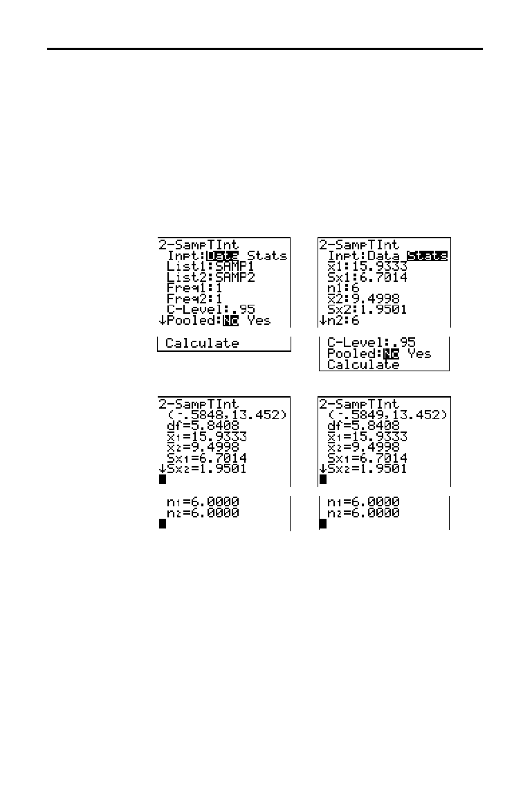
Inferential Statistics and Distributions 13-19
8313INFE.DOC TI-83 international English Bob Fedorisko Revised: 02/19/01 12:47 PM Printed: 02/19/01 1:38 PM
Page 19 of 36
2
.
SampTInt (two-sample
t
confidence interval; item 0)
computes a confidence interval for the difference between
two population means (
m
1
Nm
2
) when both population
standard deviations (
s
1
and
s
2
) are unknown. The
computed confidence interval depends on the user-
specified confidence level.
In the example:
SAMP1={12.207 16.869 25.05 22.429 8.456 10.589}
SAMP2={11.074 9.686 12.064 9.351 8.182 6.642}
Data Stats
Input:
,,
Calculated results:
2-SampTInt
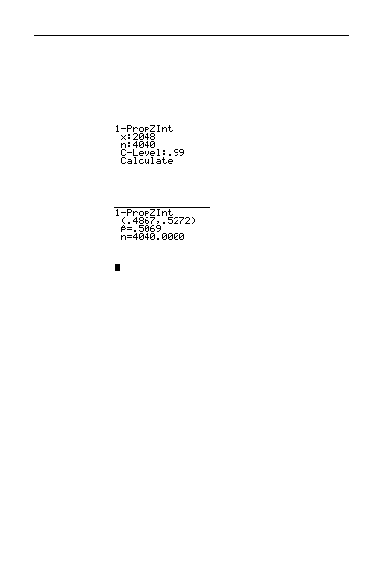
13-20 Inferential Statistics and Distributions
8313INFE.DOC TI-83 international English Bob Fedorisko Revised: 02/19/01 12:47 PM Printed: 02/19/01 1:38 PM
Page 20 of 36
1
.
PropZInt (one-proportion
z
confidence interval; item A)
computes a confidence interval for an unknown proportion
of successes. It takes as input the count of successes in the
sample
x
and the count of observations in the sample
n
.
The computed confidence interval depends on the user-
specified confidence level.
Input:
,
Calculated results:
)
1-PropZInt
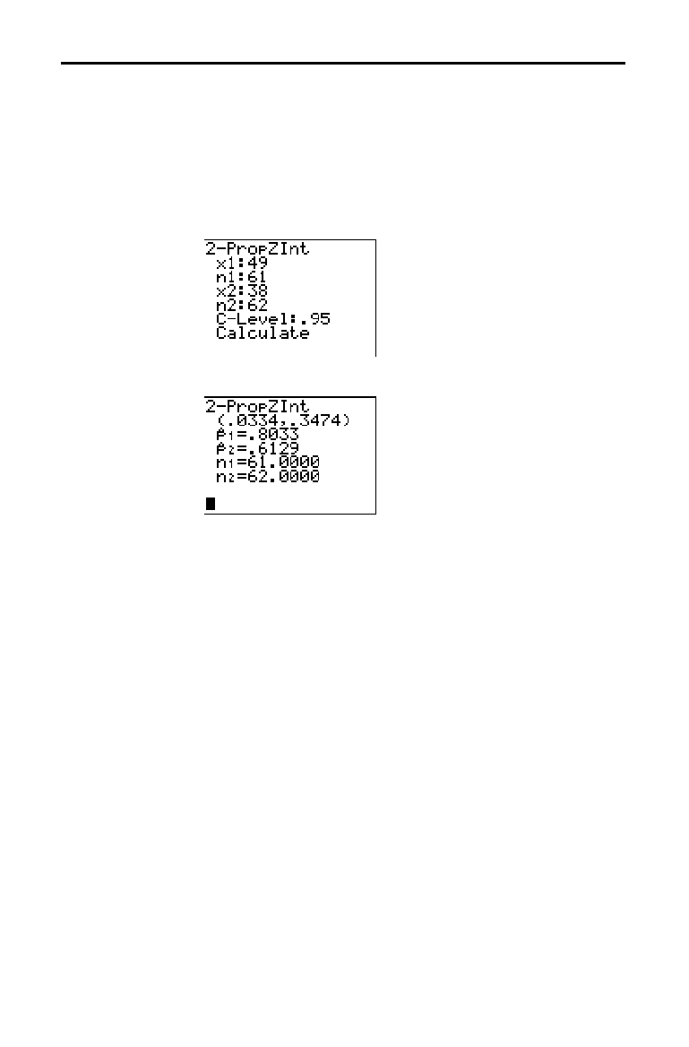
Inferential Statistics and Distributions 13-21
8313INFE.DOC TI-83 international English Bob Fedorisko Revised: 02/19/01 12:47 PM Printed: 02/19/01 1:38 PM
Page 21 of 36
2
.
PropZInt (two-proportion
z
confidence interval; item B)
computes a confidence interval for the difference between
the proportion of successes in two populations (p
1
N
p
2
). It
takes as input the count of successes in each sample
(
x
1
and
x
2
) and the count of observations in each sample
(
n
1
and
n
2
). The computed confidence interval depends on
the user-specified confidence level.
Input:
,
Calculated results:
2-PropZInt
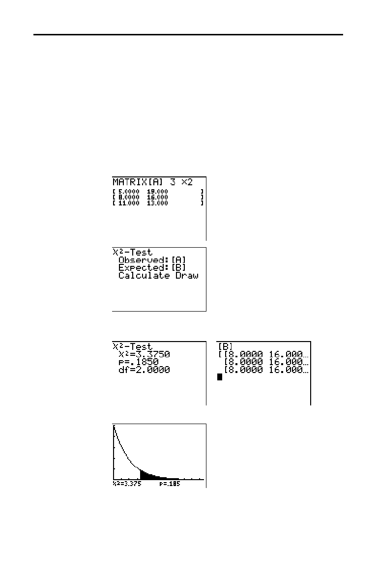
13-22 Inferential Statistics and Distributions
8313INFE.DOC TI-83 international English Bob Fedorisko Revised: 02/19/01 12:47 PM Printed: 02/19/01 1:38 PM
Page 22 of 36
c
2
.
Test
(chi-square test; item C) computes a chi-square test
for association on the two-way table of counts in the
specified
Observed
matrix. The null hypothesis H
0
for a
two-way table is: no association exists between row
variables and column variables. The alternative hypothesis
is: the variables are related.
Before computing a
c
2
.
Test, enter the observed counts in a
matrix. Enter that matrix variable name at the
Observed:
prompt in the
c
2
.
Test editor; default=
[A]. At the Expected:
prompt, enter the matrix variable name to which you want
the computed expected counts to be stored; default=
[B].
Matrix editor:
Note:
Press
~
~
1
to
select
1:[A]
from the MATRX
EDIT menu.
Input:
,
Note:
Press
[B]
Í
to
display matrix
[B]
.
Calculated results:
,
Drawn results:
c
2
-Test
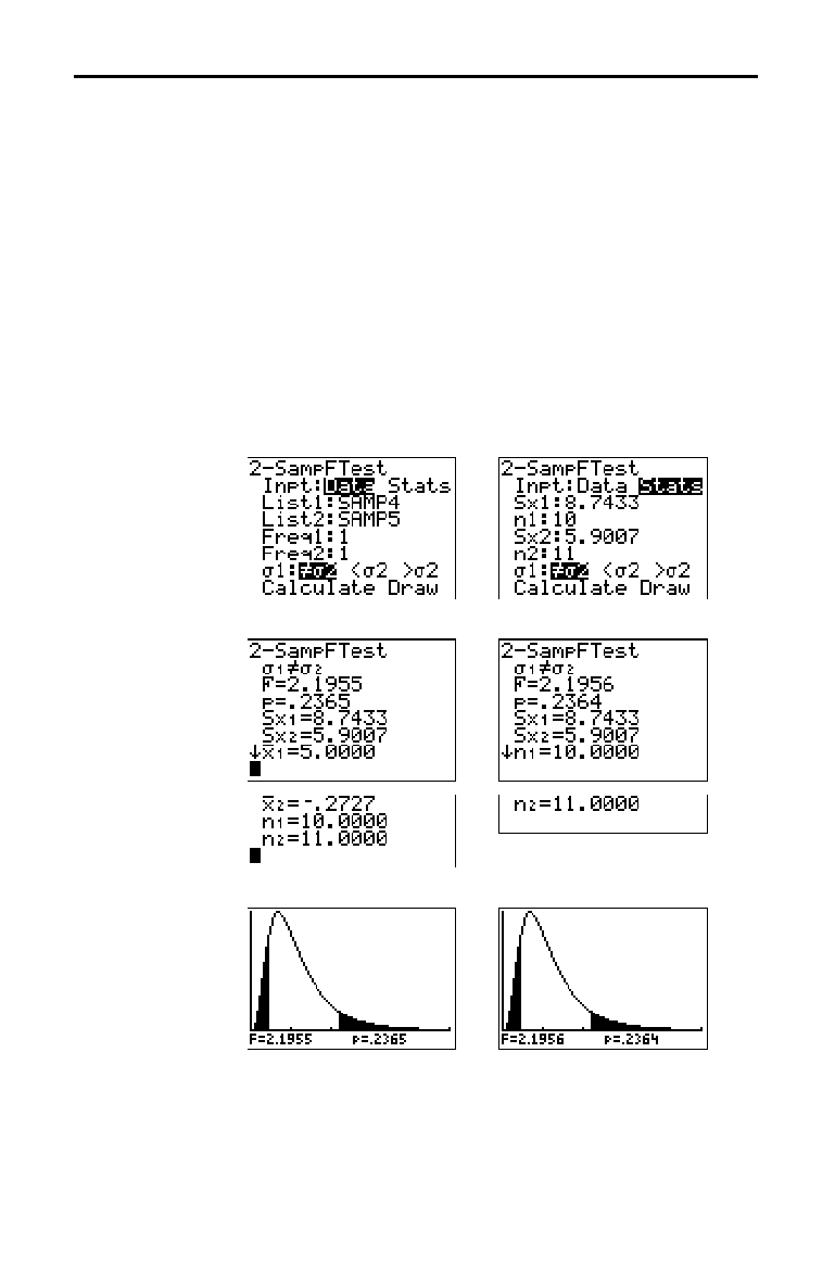
Inferential Statistics and Distributions 13-23
8313INFE.DOC TI-83 international English Bob Fedorisko Revised: 02/19/01 12:47 PM Printed: 02/19/01 1:38 PM
Page 23 of 36
2
.
Samp
Ü
Test (two-sample
Û
-test; item D) computes an
Û
-test to compare two normal population standard
deviations (
s
1
and
s
2
). The population means and standard
deviations are all unknown.
2
.
Samp
Ü
Test, which uses the
ratio of sample variances Sx1
2
/Sx2
2
, tests the null
hypothesis H
0
:
s
1
=
s
2
against one of the alternatives below.
•
H
a
:
s
1
ƒs
2
(
s
1:
ƒs
2
)
•
H
a
:
s
1
<
s
2
(
s
1:<
s
2
)
•
H
a
:
s
1
>
s
2
(
s
1:>
s
2
)
In the example:
SAMP4={ 7
L
41817
L
3
L
5 1 10 11
L
2}
SAMP5={
L
112
L
1
L
33
L
552
L
11
L
1
L
3}
Data Stats
Input:
,,
Calculated results:
,,
Drawn results:
2-Samp
Ü
Test
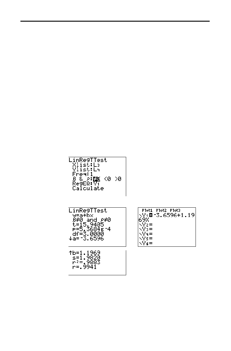
13-24 Inferential Statistics and Distributions
8313INFE.DOC TI-83 international English Bob Fedorisko Revised: 02/19/01 12:47 PM Printed: 02/19/01 1:38 PM
Page 24 of 36
LinRegTTest (linear regression
t
test; item E) computes a
linear regression on the given data and a
t
test on the value
of slope
b
and the correlation coefficient
r
for the equation
y
=
a
+
b
x. It tests the null hypothesis H
0
:
b
=0 (equivalently,
r
=0) against one of the alternatives below.
•
H
a
:
bƒ
0 and
rƒ
0 (
b
&
r
:
ƒ
0
)
•
H
a
:
b
<0 and
r
<0 (
b
&
r
:<0
)
•
H
a
:
b
>0 and
r
>0 (
b
&
r
:>0
)
The regression equation is automatically stored to
RegEQ
(
VARS Statistics EQ
secondary menu). If you enter a
Y=
variable name at the RegEQ: prompt, the calculated
regression equation is automatically stored to the specified
Y=
equation. In the example below, the regression equation
is stored to
Y
1
, which is then selected (turned on).
In the example:
L
3
={38 56 59 64 74}
L
4
={41 63 70 72 84}
Input:
,
Calculated results:
When LinRegTTest is executed, the list of residuals is
created and stored to the list name
RESID automatically.
RESID is placed on the
LIST NAMES
menu.
Note:
For the regression equation, you can use the fix-decimal mode
setting to control the number of digits stored after the decimal point
(Chapter 1). However, limiting the number of digits to a small number
could affect the accuracy of the fit.
LinRegTTest
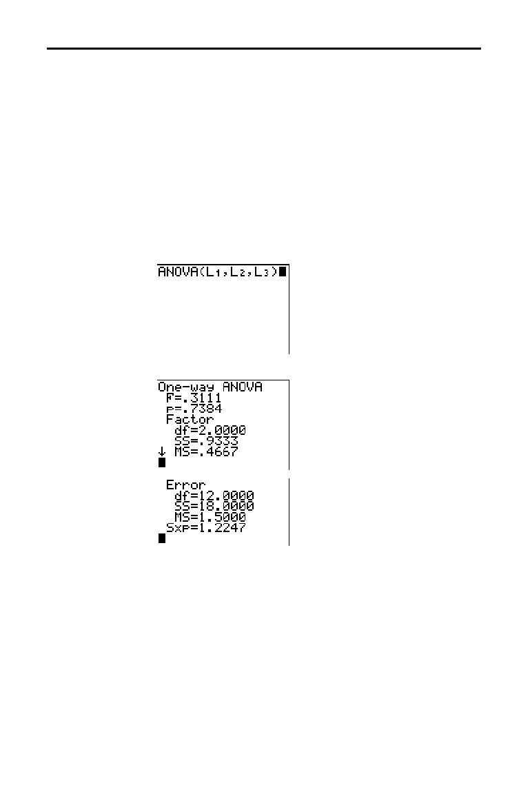
Inferential Statistics and Distributions 13-25
8313INFE.DOC TI-83 international English Bob Fedorisko Revised: 02/19/01 12:47 PM Printed: 02/19/01 1:38 PM
Page 25 of 36
ANOVA( (one-way analysis of variance; item F) computes a
one-way analysis of variance for comparing the means of
two to 20 populations. The
ANOVA
procedure for
comparing these means involves analysis of the variation
in the sample data. The null hypothesis H
0
:
m
1
=
m
2
=...=
m
k
is
tested against the alternative H
a
: not all
m
1
...
m
k
are equal.
ANOVA(
list1
,
list2
[
,
...
,
list20
]
)
In the example:
L
1
={7 4 6 6 5}
L
2
={6 5 5 8 7}
L
3
={4 7 6 7 6}
Input:
,
Calculated results:
Note:
SS
is sum of squares and
MS
is mean square.
ANOVA(

13-26 Inferential Statistics and Distributions
8313INFE.DOC TI-83 international English Bob Fedorisko Revised: 02/19/01 12:47 PM Printed: 02/19/01 1:38 PM
Page 26 of 36
The tables in this section describe the inferential statistics inputs discussed in
this chapter. You enter values for these inputs in the inferential stat editors.
The tables present the inputs in the same order that they appear in this
chapter.
Input Description
m
0
Hypothesized value of the population mean that you are
testing.
s
The known population standard deviation; must be a real
number > 0.
List
The name of the list containing the data you are testing.
Freq
The name of the list containin
g
the frequency values for the
data in
List
. Default=1. All elements must be integers
|
0.
Calculate
/
Draw
Determines the type of output to
g
enerate for tests and
intervals.
Calculate
displays the output on the home screen.
In tests,
Draw
draws a graph of the results.
v
,
Sx
,
n
Summary statistics
(
mean, standard deviation, and sample
size) for the one-sample tests and intervals.
s
1
The known population standard deviation from the first
population for the two-sample tests and intervals. Must be
a real number > 0.
s
2
The known population standard deviation from the second
population for the two-sample tests and intervals. Must be
a real number > 0.
List1
,
List2
The names of the lists containin
g
the data you are testin
g
for the two-sample tests and intervals. Defaults are
L
1
and
L
2
, respectively.
Freq1
,
Freq2
The names of the lists containin
g
the frequencies for the
data in
List1
and
List2
for the two-sample tests and
intervals. Defaults=1. All elements must be integers
|
0.
v
1
,
Sx1
,
n
1
,
v
2
,
Sx2
,
n
2
Summary statistics
(
mean, standard deviation, and sample
size
)
for sample one and sample two in the two-sample
tests and intervals.
Pooled
Specifies whether variances are to be pooled for
2
.
SampTTest
and
2
.
SampTInt
.
No
instructs the TI
.
83 not to
pool the variances.
Yes
instructs the TI
.
83 to pool the
v
ariances.
Inferential Statistics Input Descriptions

Inferential Statistics and Distributions 13-27
8313INFE.DOC TI-83 international English Bob Fedorisko Revised: 02/19/01 12:47 PM Printed: 02/19/01 1:38 PM
Page 27 of 36
Input Description
p
0
The expected sample proportion for
1
.
PropZTest
. Must be
a
real number, such that 0 <
p
0
< 1.
x
The count of successes in the sample for the
1
.
PropZTest
and
1
.
PropZInt
. Must be an integer
‚
0.
n
The count of observations in the sample for the
1
.
PropZTest
and
1
.
PropZInt
. Must be an integer > 0.
x1
The count of successes from sample one for the
2
.
PropZTest
and
2
.
PropZInt
. Must be an integer
‚
0.
x2
The count of successes from sample two for the
2
.
PropZTest
and
2
.
PropZInt
. Must be an integer
‚
0.
n1
The count of observations in sample one for the
2
.
PropZTest
and
2
.
PropZInt
. Must be an integer > 0.
n2
The count of observations in sample two for the
2
.
PropZTest
and
2
.
PropZInt
. Must be an integer > 0.
C
.
Level
The confidence level for the interval instructions. Must be
‚
0 and <100. If it is
‚
1, it is assumed to be given as a
percent and is divided by 100. Default=0.95.
Observed (Matrix)
The matrix name that represents the columns and rows for
the observed values of a two-way table of counts for the
c
2
.
Test
.
Observed
must contain all integers
‚
0. Matrix
dimensions must be at least 2×2.
Expected (Matrix)
The matrix name that specifies where the expected values
should be stored.
Expected
is created upon successful
completion of the
c
2
.
Test
.
Xlist
,
Ylist
The names of the lists containing the data for
LinRegTTest
.
Defaults are
L
1
and
L
2
, respectively. The dimensions of
Xlist
and
Ylist
must be the same.
RegEQ
The prompt for the name of the
Y=
variable where the
calculated regression equation is to be stored. If a
Y=
variable is specified, that equation is automatically
selected (turned on). The default is to store the regression
equation to the
RegEQ
variable only.

13-28 Inferential Statistics and Distributions
8313INFE.DOC TI-83 international English Bob Fedorisko Revised: 02/19/01 12:47 PM Printed: 02/19/01 1:38 PM
Page 28 of 36
The inferential statistics variables are calculated as indicated below. To access
these variables for use in expressions, press
,
5 (5:Statistics), and then
select the
VARS
menu listed in the last column below.
Variables Tests Intervals
LinRegTTest,
ANOVA
VARS
Menu
p-value pp
TEST
test statistics z, t,
c
2
,
Ü
t
,
Ü
TEST
degrees of freedom df df df
TEST
sample mean of x values for
sample 1 and sample 2
v
1
,
v
2
v
1
,
v
2
TEST
sample standard deviation of x
for sample 1 and sample 2
Sx1,
Sx2
Sx1,
Sx2
TEST
number of data points for sample
1 and sample 2
n1, n2 n1, n2
TEST
pooled standard deviation SxP SxP SxP
TEST
estimated sample proportion
ÇÇ
TEST
estimated sample proportion for
population 1
Ç
1
Ç
1
TEST
estimated sample proportion for
population 2
Ç
2
Ç
2
TEST
confidence interval pair lower,
upper
TEST
mean of x values
vv
XY
sample standard deviation of x Sx Sx
XY
number of data points nn
XY
standard error about the line s
TEST
regression/fit coefficients a, b
EQ
correlation coefficient r
EQ
coefficient of determination r
2
EQ
regression equation RegEQ
EQ
Test and Interval Output Variables
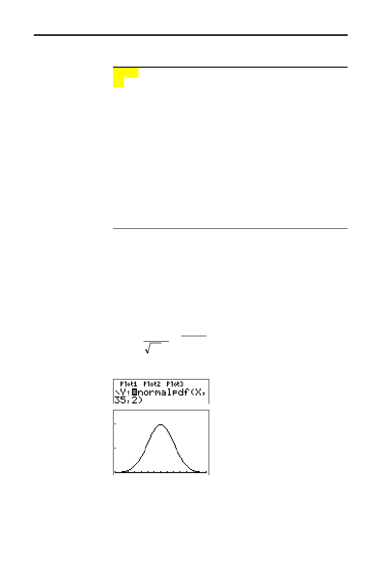
Inferential Statistics and Distributions 13-29
8313INFE.DOC TI-83 international English Bob Fedorisko Revised: 02/19/01 12:47 PM Printed: 02/19/01 1:38 PM
Page 29 of 36
To display the
DISTR
menu, press
y
[
DISTR
].
DISTR DRAW
1: normalpdf(
Normal probability density
2: normalcdf(
Normal distribution probability
3: invNorm(
Inverse cumulative normal distribution
4: tpdf(
Student-
t
probability density
5: tcdf(
Student-
t
distribution probability
6:
c
2
pdf(
Chi-square probability density
7:
c
2
cdf
Chi-square distribution probability
8:
Ü
pdf( Û
probability density
9:
Ü
cdf( Û
distribution probability
0: binompdf(
Binomial probability
A: binomcdf(
Binomial cumulative density
B: poissonpdf(
Poisson probability
C: poissoncdf(
Poisson cumulative density
D: geometpdf(
Geometric probability
E: geometcdf(
Geometric cumulative density
Note:
L
1
å
99 and 1
å
99 specify infinity. If you want to view the area left
of
upperbound
, for example, specify
lowerbound
=
L
1
å
99.
norwmalpdf(
computes the probability density function
(pdf) for the normal distribution at a specified
x
value. The
defaults are mean
m
=0 and standard deviation
s
=1. To plot
the normal distribution, paste
normalpdf(
to the
Y=
editor.
The probability density function (pdf) is:
fx e
x
()
=>
−
−
1
2
0
2
2
2
πσ
σ
µ
σ
()
,
normalpdf(
x
[
,
m
,
s
]
)
Note:
For this example,
Xmin = 28
Xmax = 42
Ymin = 0
Ymax = .25
Tip:
For plotting the normal distribution, you can set window variables
Xmin
and
Xmax
so that the mean
m
falls between them, and then
select
0:ZoomFit
from the
ZOOM
menu.
Distribution Functions
DISTR menu
normalpdf(
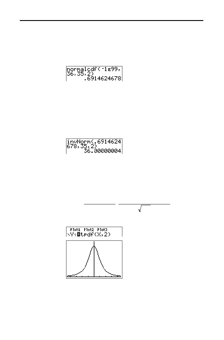
13-30 Inferential Statistics and Distributions
8313INFE.DOC TI-83 international English Bob Fedorisko Revised: 02/19/01 12:47 PM Printed: 02/19/01 1:38 PM
Page 30 of 36
normalcdf( computes the normal distribution probability
between
lowerbound
and
upperbound
for the specified
mean
m
and standard deviation
s
. The defaults are
m
=0
and
s
=1.
normalcdf(
lowerbound
,
upperbound
[
,
m
,
s
])
invNorm( computes the inverse cumulative normal
distribution function for a given
area
under the normal
distribution curve specified by mean
m
and standard
deviation
s
. It calculates the
x
value associated with an
area
to the left of the
x
value. 0
area
1 must be true.
The defaults are
m
=0 and
s
=1.
invNorm(
area
[
,
m
,
s
])
tpdf( computes the probability density function (pdf) for
the Student-
t
distribution at a specified
x
value.
df
(degrees
of freedom) must be >0. To plot the Student-
t
distribution,
paste
tpdf( to the
Y=
editor. The probability density
function (pdf) is:
fx
df
df
xdf
df
df
()
[( ) ]
()
()
()
=
++
−+
Γ
Γ
12
2
1
2
12
/
/
/
/
π
tpdf(
x
,
df
)
Note:
For this example,
Xmin =
L
4.5
Xmax = 4.5
Ymin = 0
Ymax = .4
normalcdf(
invNorm(
tpdf(
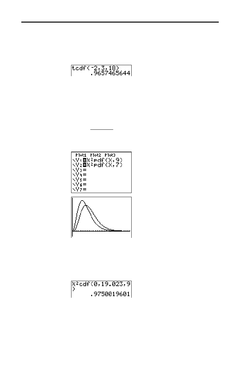
Inferential Statistics and Distributions 13-31
8313INFE.DOC TI-83 international English Bob Fedorisko Revised: 02/19/01 12:47 PM Printed: 02/19/01 1:38 PM
Page 31 of 36
tcdf( computes the Student-
t
distribution probability
between
lowerbound
and
upperbound
for the specified
df
(degrees of freedom), which must be > 0.
tcdf(
lowerbound
,
upperbound
,
df
)
c
2
pdf( computes the probability density function (pdf) for
the
c
2
(chi-square) distribution at a specified
x
value.
df
(degrees of freedom) must be an integer > 0. To plot the
c
2
distribution, paste
c
2
pdf( to the
Y=
editor. The probability
density function (pdf) is:
fx
df
xex
df df x
()
()
(1/2)=≥
−−
1
2
0
221 2
Γ
/
,
// /
c
2
pdf(
x
,
df
)
Note:
For this example,
Xmin = 0
Xmax = 30
Ymin =
L
.02
Ymax = .132
c
2
cdf( computes the
c
2
(chi-square) distribution probability
between
lowerbound
and
upperbound
for the specified
df
(degrees of freedom), which must be an integer > 0.
c
2
cdf(
lowerbound
,
upperbound
,
df
)
tcdf(
c
2
pdf(
c
2
cdf(
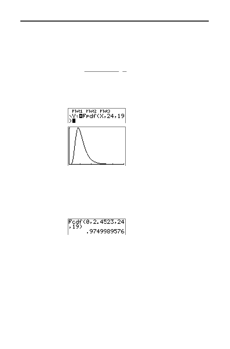
13-32 Inferential Statistics and Distributions
8313INFE.DOC TI-83 international English Bob Fedorisko Revised: 02/19/01 12:47 PM Printed: 02/19/01 1:38 PM
Page 32 of 36
Ü
pdf(
computes the probability density function (pdf) for
the
Û
distribution at a specified
x
value.
numerator df
(degrees of freedom) and
denominator df
must be integers
> 0. To plot the
Û
distribution, paste
Ü
pdf(
to the
Y=
editor.
The probability density function (pdf) is:
fx
nd
nd
n
d
xnxd x
n
nnd
()
[( ) ]
()()
()
()
=
+
+≥
−−+
Γ
ΓΓ
/
//
/,
/
//
2
22
10
2
21 2
where
n
= numerator degrees of freedom
d
= denominator degrees of freedom
Ü
pdf(
x
,
numerator df
,
denominator df
)
Note:
For this example,
Xmin = 0
Xmax = 5
Ymin = 0
Ymax = 1
Ü
cdf(
computes the
Û
distribution probability between
lowerbound
and
upperbound
for the specified
numerator
df
(degrees of freedom) and
denominator df
.
numerator
df
and
denominator df
must be integers >0.
Ü
cdf(
lowerbound
,
upperbound
,
numerator df
,
denominator df
)
Ü
pdf(
Ü
cdf(
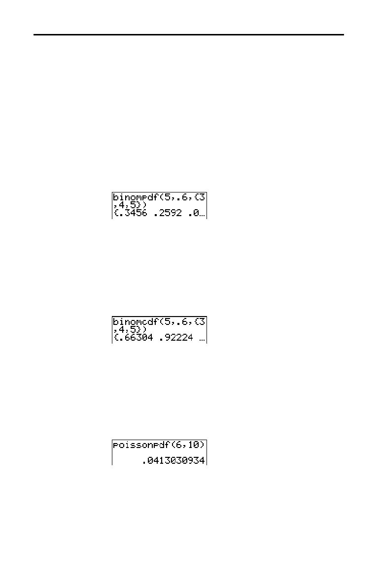
Inferential Statistics and Distributions 13-33
8313INFE.DOC TI-83 international English Bob Fedorisko Revised: 02/19/01 12:47 PM Printed: 02/19/01 1:38 PM
Page 33 of 36
binompdf( computes a probability at
x
for the discrete
binomial distribution with the specified
numtrials
and
probability of success (
p
) on each trial.
x
can be an integer
or a list of integers. 0
p
1 must be true.
numtrials
must be
an integer > 0. If you do not specify
x
, a list of probabilities
from 0 to
numtrials
is returned. The probability density
function (pdf) is:
fx
n
x
pp x n
xnx
() ( )
=
−=
−
101
,,,,
where
n = numtrials
binompdf(
numtrials
,
p
[
,
x
]
)
binomcdf( computes a cumulative probability at
x
for the
discrete binomial distribution with the specified
numtrials
and probability of success (
p
) on each trial.
x
can be a real
number or a list of real numbers. 0
p
1 must be true.
numtrials
must be an integer > 0. If you do not specify
x
, a
list of cumulative probabilities is returned.
binomcdf(
numtrials
,
p
[
,
x
]
)
poissonpdf( computes a probability at
x
for the discrete
Poisson distribution with the specified mean
m
, which must
be a real number > 0.
x
can be an integer or a list of
integers. The probability density function (pdf) is:
fx e x x
x
() !==
−µ
µ
/, ,,,
012
poissonpdf(
m
,
x
)
binompdf(
binomcdf(
poissonpdf(
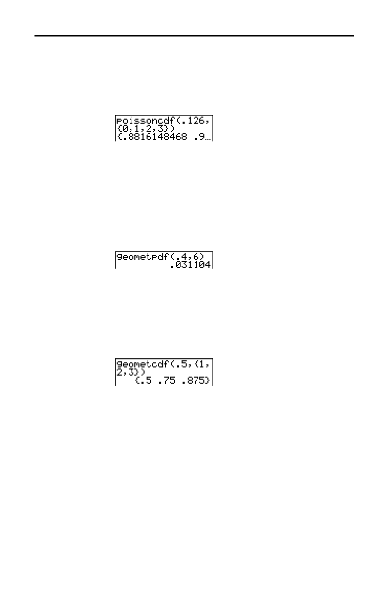
13-34 Inferential Statistics and Distributions
8313INFE.DOC TI-83 international English Bob Fedorisko Revised: 02/19/01 12:47 PM Printed: 02/19/01 1:38 PM
Page 34 of 36
poissoncdf( computes a cumulative probability at
x
for the
discrete Poisson distribution with the specified mean
m
,
which must be a real number > 0.
x
can be a real number
or a list of real numbers.
poissoncdf(
m
,
x
)
geometpdf( computes a probability at
x
, the number of the
trial on which the first success occurs, for the discrete
geometric distribution with the specified probability of
success
p
. 0
p
1 must be true.
x
can be an integer or a list
of integers. The probability density function (pdf) is:
fx p p x
x
() ( )
=− =
−
112
1
,,,
geometpdf(
p
,
x
)
geometcdf( computes a cumulative probability at
x
, the
number of the trial on which the first success occurs, for
the discrete geometric distribution with the specified
probability of success
p
. 0
p
1 must be true.
x
can be a
real number or a list of real numbers.
geometcdf(
p
,
x
)
poissoncdf(
geometpdf(
geometcdf(
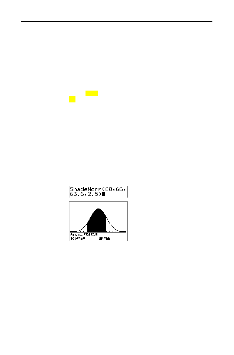
Inferential Statistics and Distributions 13-35
8313INFE.DOC TI-83 international English Bob Fedorisko Revised: 02/19/01 12:47 PM Printed: 02/19/01 1:38 PM
Page 35 of 36
To display the
DISTR DRAW
menu, press
y
[
DISTR
]
~
.
DISTR DRAW
instructions draw various types of density
functions, shade the area specified by
lowerbound
and
upperbound
, and display the computed area value.
To clear the drawings, select
1:ClrDraw from the
DRAW
menu (Chapter 8).
Note
: Before you execute a
DISTR DRAW
instruction, you must set
the window variables so that the desired distribution fits the screen.
DISTR DRAW
1: ShadeNorm(
Shades normal distribution.
2:Shade_t(
Shades Student-
t
distribution.
3:Shade
c
2
(
Shades
c
2
distribution.
4:Shade
Û
(
Shades
Û
distribution.
Note:
L
1
å
99 and 1
å
99 specify infinity. If you want to view the area left
of
upperbound
, for example, specify
lowerbound
=
L
1
å
99.
ShadeNorm( draws the normal density function specified
by mean
m
and standard deviation
s
and shades the area
between
lowerbound
and
upperbound
. The defaults are
m
=0 and
s
=1.
ShadeNorm(
lowerbound
,
upperbound
[
,
m
,
s
]
)
Note:
For this example,
Xmin = 55
Xmax = 72
Ymin =
L
.05
Ymax = .2
Distribution Shading
DISTR DRAW
Menu
ShadeNorm(
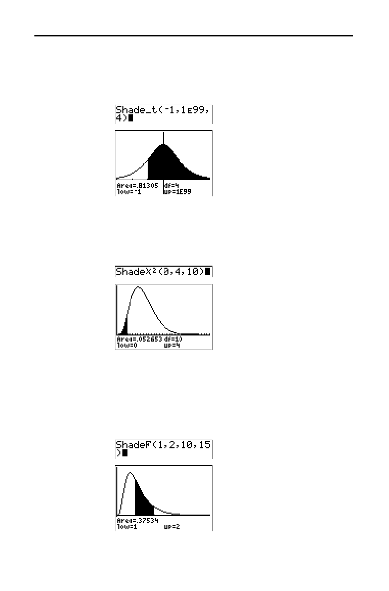
13-36 Inferential Statistics and Distributions
8313INFE.DOC TI-83 international English Bob Fedorisko Revised: 02/19/01 12:47 PM Printed: 02/19/01 1:38 PM
Page 36 of 36
Shade_t( draws the density function for the Student-
t
distribution specified by
df
(degrees of freedom) and
shades the area between
lowerbound
and
upperbound
.
Shade_t(
lowerbound
,
upperbound
,
df
)
Note:
For this example,
Xmin =
L
3
Xmax = 3
Ymin =
L
.15
Ymax = .5
Shade
c
2
( draws the density function for the
c
2
(chi-square)
distribution specified by
df
(degrees of freedom) and shades
the area between
lowerbound
and
upperbound
.
Shade
c
2
(
lowerbound
,
upperbound
,
df
)
Note:
For this example,
Xmin = 0
Xmax = 35
Ymin =
L
.025
Ymax = .1
Shade
Ü
(
draws the density function for the
Û
distribution
specified by
numerator df
(degrees of freedom)
and
denominator df
and shades the area between
lowerbound
and
upperbound
.
Shade
Ü
(
lowerbound
,
upperbound
,
numerator df
,
denominator df
)
Note:
For this example,
Xmin = 0
Xmax = 5
Ymin =
L
.25
Ymax = .9
Shade_t(
Shade
c
2
(
Shade
Ü
(
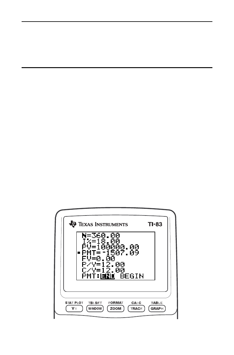
Financial Functions 14-1
8314FINA.DOC TI-83 international English Bob Fedorisko Revised: 02/19/01 12:50 PM Printed: 02/19/01 1:38 PM
Page 1 of 14
14
Financial
Functions
Getting Started: Financing a Car
.........................
14-2
Getting Started: Computing Compound Interest
..........
14-3
Using the
TVM Solver
....................................
14-4
Using the Financial Functions
...........................
14-5
Calculating Time Value of Money (
TVM
)
.................
14-6
Calculating Cash Flows
..................................
14-8
Calculating Amortization
................................
14-9
Calculating Interest Conversion
..........................
14-12
Finding Days between Dates/Defining Payment Method
.....
14-13
Using the
TVM
Variables
.................................
14-14
Contents
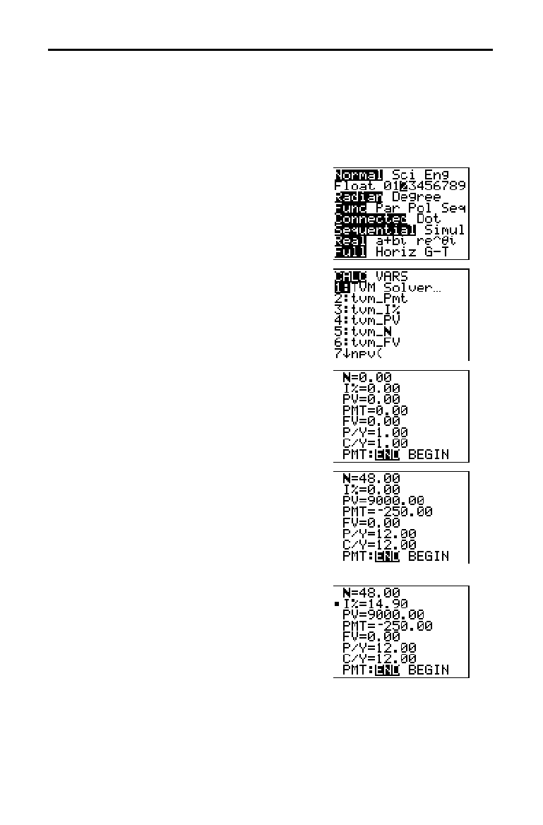
14-2 Financial Functions
8314FINA.DOC TI-83 international English Bob Fedorisko Revised: 02/19/01 12:50 PM Printed: 02/19/01 1:38 PM
Page 2 of 14
Getting Started is a fast-paced introduction. Read the chapter for details.
You have found a car you would like to buy. The car costs 9,000. You can
afford payments of 250 per month for four years. What annual percentage rate
(APR) will make it possible for you to afford the car?
1. Press
z
†
~
~
~
Í
to set the
fixed-decimal mode setting to
2. The TI
-
83
will display all numbers with two decimal
places.
2. Press
y
[
FINANCE
] to display the
FINANCE CALC
menu.
3. Press
Í
to select 1:TVM Solver. The
TVM Solver
is displayed.
Press
48
Í
to store 48 months to
Ú
.
Press
†
9000
Í
to store 9,000 to PV.
Press
Ì
250
Í
to store
L
250 to PMT.
(Negation indicates cash outflow.) Press
0
Í
to store 0 to
FV. Press 12
Í
to
store 12 payments per year to
P/Y and 12
compounding periods per year to
C/Y.
Setting
P/Y to 12 will compute an annual
percentage rate (compounded monthly)
for
æ
. Press
†
Í
to select PMT:END,
which indicates that payments are due at
the end of each period.
4. Press
}
}
}
}
}
}
to move the cursor
to the
æ
prompt. Press
ƒ
[
SOLVE
] to
solve for
æ
. What APR should you look
for?
Getting Started: Financing a Car
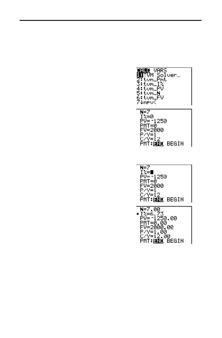
Financial Functions 14-3
8314FINA.DOC TI-83 international English Bob Fedorisko Revised: 02/19/01 12:50 PM Printed: 02/19/01 1:38 PM
Page 3 of 14
At what annual interest rate, compounded monthly, will 1,250 accumulate to
2,000 in 7 years?
Note:
Because there are no payments when you solve compound interest problems,
PMT
must be set to
0
and
P/Y
must be
set to
1
.
1. Press
y
[
FINANCE
] to display the
FINANCE CALC
menu.
2. Press
Í
to select
1:TVM Solver
. Press
7
to enter the number of periods in years.
Press
†
†
Ì
1250
to enter the present
value as a cash outflow (investment).
Press
†
0
to specify no payments. Press
†
2000
to enter the future value as a cash
inflow (return). Press
†
1
to enter
payment periods per year. Press
†
12
to
set compounding periods per year to
12
.
3. Press
}
}
}
}
}
to place the cursor on
the
æ
prompt.
4. Press
ƒ
[
SOLVE
] to solve for
æ
, the
annual interest rate.
Getting Started: Computing Compound Interest
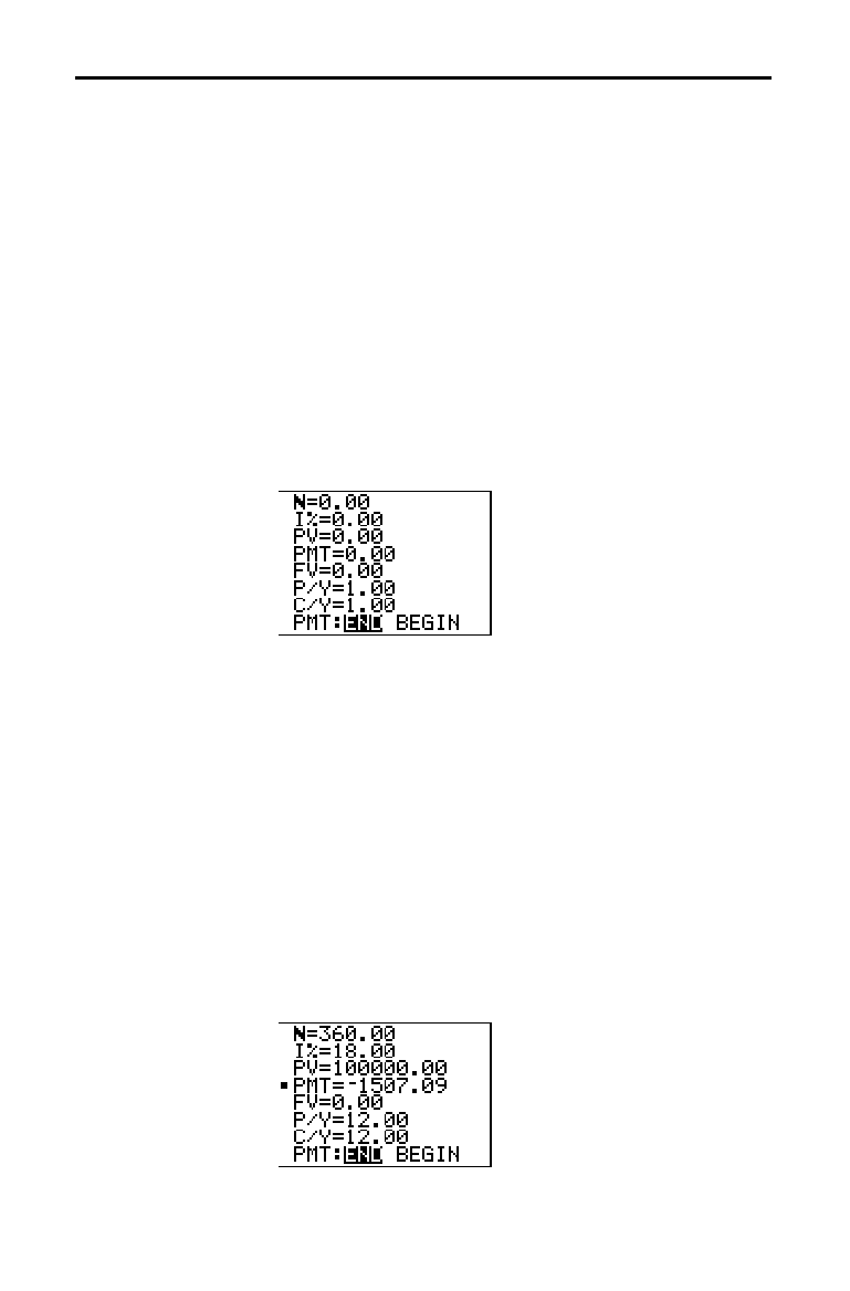
14-4 Financial Functions
8314FINA.DOC TI-83 international English Bob Fedorisko Revised: 02/19/01 12:50 PM Printed: 02/19/01 1:38 PM
Page 4 of 14
The
TVM Solver
displays the time-value-of-money (
TVM
)
variables. Given four variable values, the
TVM Solver
solves
for the fifth variable.
The
FINANCE VARS
menu section (page 14
.
14) describes
the five
TVM
variables (
Ú
,
æ
, PV, PMT, and FV) and P/Y and
C/Y.
PMT: END BEGIN in the
TVM Solver
corresponds to the
FINANCE CALC
menu items Pmt_End (payment at the end
of each period) and
Pmt_Bgn (payment at the beginning of
each period).
To solve for an unknown
TVM
variable, follow these steps.
1. Press
y
[
FINANCE
]
Í
to display the
TVM Solver
. The
screen below shows the default values with the fixed-
decimal mode set to two decimal places.
2. Enter the known values for four
TVM
variables.
Note
: Enter cash inflows as positive numbers and cash
outflows as negative numbers.
3. Enter a value for P/Y, which automatically enters the
same value for
C/Y; if P/Y
ƒ
C/Y, enter a unique value for
C/Y.
4. Select
END or BEGIN to specify the payment method.
5. Place the cursor on the
TVM
variable for which you
want to solve.
6. Press
ƒ
[
SOLVE
]. The answer is computed,
displayed in the
TVM Solver
, and stored to the
appropriate
TVM
variable. An indicator square in the left
column designates the solution variable.
Using the TVM Solver
Using the TVM
Solver

Financial Functions 14-5
8314FINA.DOC TI-83 international English Bob Fedorisko Revised: 02/19/01 12:50 PM Printed: 02/19/01 1:38 PM
Page 5 of 14
When using the TI
-
83 financial functions, you must enter
cash inflows (cash received) as positive numbers and cash
outflows (cash paid) as negative numbers. The TI
-
83
follows this convention when computing and displaying
answers.
To display the
FINANCE CALC
menu, press
y
[
FINANCE
].
CALC VARS
1: TVM Solver
...
Displays the
TVM Solver.
2: tvm_Pmt
Computes the amount of each payment.
3: tvm_
æ
Computes the interest rate per year.
4: tvm_PV
Computes the present value.
5: tvm_
Ú
Computes the number of payment periods.
6: tvm_FV
Computes the future value.
7: npv(
Computes the net present value.
8: irr(
Computes the internal rate of return.
9: bal(
Computes the amortization sched. balance.
0:
G
Prn(
Computes the amort. sched. principal sum.
A:
G
Int(
Computes the amort. sched. interest sum.
B:
4
Nom(
Computes the nominal interest rate.
C:
4
Eff(
Computes the effective interest rate.
D: dbd(
Calculates the days between two dates.
E: Pmt_End
Selects ordinary annuity (end of period).
F: Pmt_Bgn
Selects annuity due (beginning of period).
Use these functions to set up and perform financial
calculations on the home screen.
TVM Solver
displays the
TVM Solver
(page 14
.
4).
Using the Financial Functions
Entering Cash
Inflows and Cash
Outflows
FINANCE CALC
Menu
TVM Solver
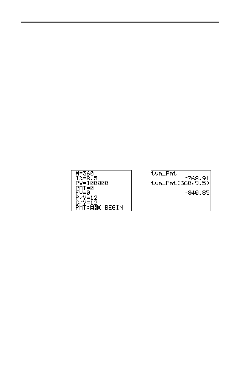
14-6 Financial Functions
8314FINA.DOC TI-83 international English Bob Fedorisko Revised: 02/19/01 12:50 PM Printed: 02/19/01 1:38 PM
Page 6 of 14
Use time-value-of-money (
TVM
) functions (menu items 2
through 6) to analyze financial instruments such as
annuities, loans, mortgages, leases, and savings.
Each
TVM
function takes zero to six arguments, which
must be real numbers. The values that you specify as
arguments for these functions are not stored to the
TVM
variables (page 14
.
14).
Note:
To store a value to a
TVM
variable, use the
TVM Solver
(page
14
.
4) or use
¿
and any
TVM
variable on the
FINANCE VARS
menu (page 14
.
14).
If you enter less than six arguments, the TI
-
83 substitutes a
previously stored
TVM
variable value for each unspecified
argument.
If you enter any arguments with a
TVM
function, you must
place the argument or arguments in parentheses.
tvm_Pmt computes the amount of each payment.
tvm_Pmt[(
Ú
,
æ
,
PV
,
FV
,
P/Y
,
C/Y
)]
Note:
In the example above, the values are stored to the
TVM
variables in the
TVM Solver
. Then the payment (
tvm_Pmt
) is
computed on the home screen using the values in the
TVM Solver
.
Next, the interest rate is changed to 9.5 to illustrate the effect on the
payment amount.
Calculating Time Value of Money (TVM)
Calculating Time
Value of Money
tvm_Pmt
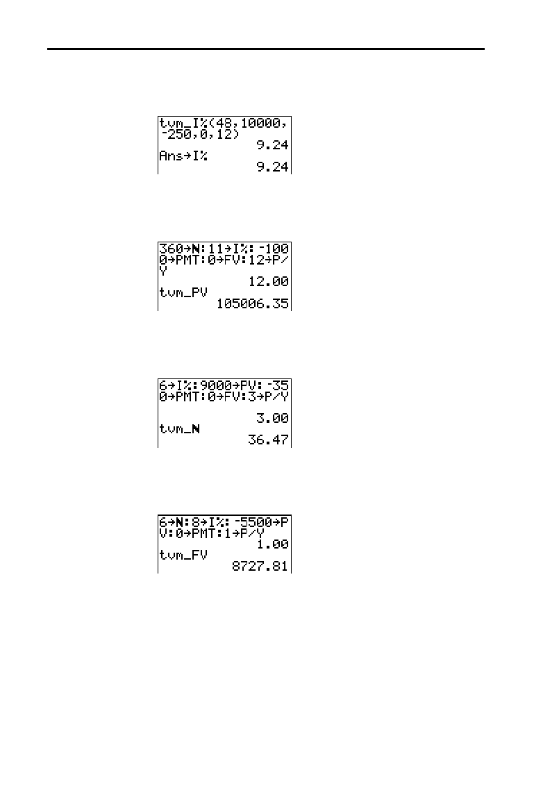
Financial Functions 14-7
8314FINA.DOC TI-83 international English Bob Fedorisko Revised: 02/19/01 12:50 PM Printed: 02/19/01 1:38 PM
Page 7 of 14
tvm_
æ
computes the annual interest rate.
tvm_
æ
[(
Ú
,
PV
,
PMT
,
FV
,
P/Y
,
C/Y
)]
tvm_PV computes the present value.
tvm_PV[(
Ú
,
æ
,
PMT
,
FV
,
P/Y
,
C/Y
)]
tvm_
Ú
computes the number of payment periods.
tvm_
Ú
[(
æ
,
PV
,
PMT
,
FV
,
P/Y
,
C/Y
)]
tvm_FV computes the future value.
tvm_FV[(
Ú
,
æ
,
PV
,
PMT
,
P/Y
,
C/Y
)]
tvm_
æ
tvm_PV
tvm_
Ú
tvm_FV
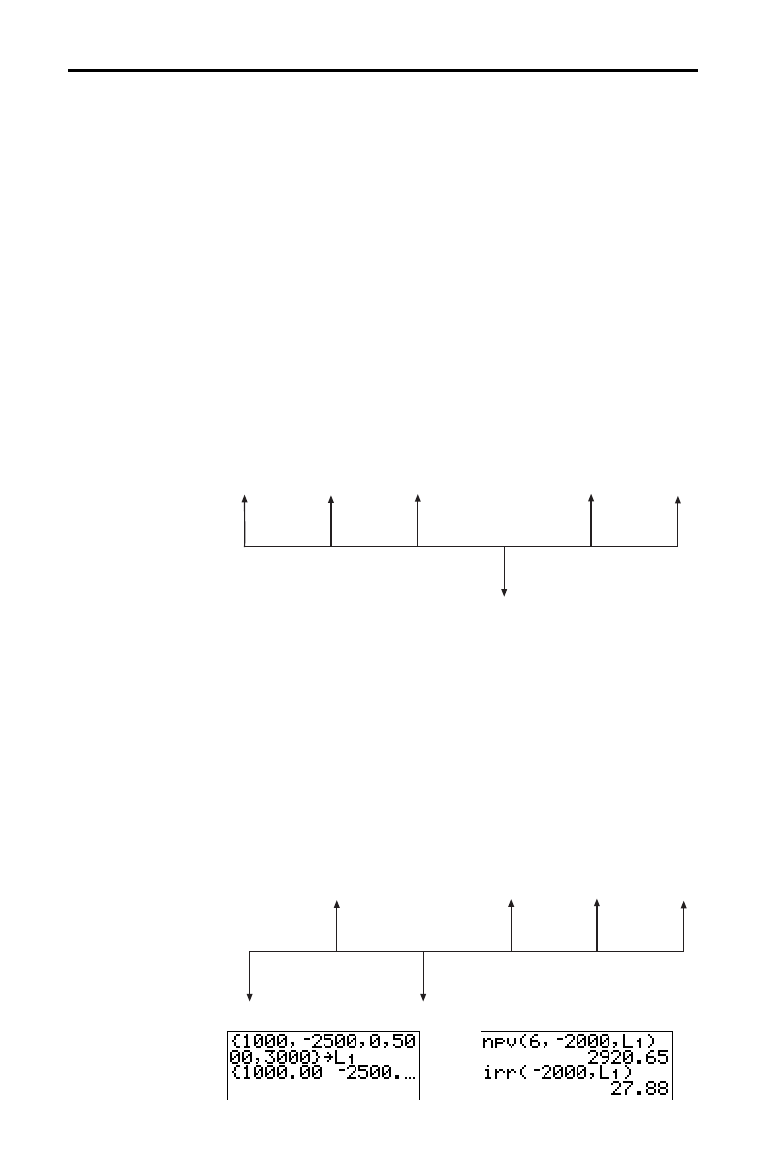
14-8 Financial Functions
8314FINA.DOC TI-83 international English Bob Fedorisko Revised: 02/19/01 12:50 PM Printed: 02/19/01 1:38 PM
Page 8 of 14
Use the cash flow functions (menu items 7 and 8) to
analyze the value of money over equal time periods. You
can enter unequal cash flows, which can be cash inflows or
outflows. The syntax descriptions for
npv(
and irr(
use
these arguments.
•
interest rate
is the rate by which to discount the cash
flows (the cost of money) over one period.
•
CF0
is the initial cash flow at time 0; it must be a real
number.
•
CFList
is a list of cash flow amounts after the initial
cash flow
CF0
.
•
CFFreq
is a list in which each element specifies the
frequency of occurrence for a grouped (consecutive)
cash flow amount, which is the corresponding element
of
CFList
. The default is 1; if you enter values, they
must be positive integers < 10,000.
For example, express this uneven cash flow in lists.
2000
4000
2000
2000
- 3000
4000
CF0
=
2000
CFList
=
{2000,
L
3000,4000}
CFFreq
=
{2,1,2}
npv(
(net present value) is the sum of the present values
for the cash inflows and outflows. A positive result for
npv
indicates a profitable investment.
npv(
interest rate
,
CF0
,
CFList
[
,
CFFreq
]
)
irr( (internal rate of return) is the interest rate at which the
net present value of the cash flows is equal to zero.
irr(
CF0
,
CFList
[
,
CFFreq
]
)
3000
5000
1000
- 2000
- 2500
0
Calculating Cash Flows
Calculating a
Cash Flow
npv(, irr(

Financial Functions 14-9
8314FINA.DOC TI-83 international English Bob Fedorisko Revised: 02/19/01 12:50 PM Printed: 02/19/01 1:38 PM
Page 9 of 14
Use the amortization functions (menu items 9, 0, and A) to
calculate balance, sum of principal, and sum of interest for
an amortization schedule.
bal( computes the balance for an amortization schedule
using stored values for
æ
, PV, and PMT.
npmt
is the
number of the payment at which you want to calculate a
balance. It must be a positive integer < 10,000.
roundvalue
specifies the internal precision the calculator uses to
calculate the balance; if you do not specify
roundvalue
,
then the TI
-
83 uses the current
Float/Fix decimal-mode
setting.
bal(
npmt
[
,
roundvalue
]
)
G
Prn(
computes the sum of the principal during a specified
period for an amortization schedule using stored values for
æ
, PV, and PMT.
pmt1
is the starting payment.
pmt2
is the
ending payment in the range.
pmt1
and
pmt2
must be
positive integers < 10,000.
roundvalue
specifies the internal
precision the calculator uses to calculate the principal; if you
do not specify
roundvalue
, the TI
-
83 uses the current
Float/Fix decimal-mode setting.
Note:
You must enter values for
æ
,
PV
,
PMT
, and before computing
the principal.
G
Prn(
pmt1
,
pmt2
[
,
roundvalue
]
)
G
Int( computes the sum of the interest during a specified
period for an amortization schedule using stored values for
æ
, PV, and PMT.
pmt1
is the starting payment.
pmt2
is the
ending payment in the range.
pmt1
and
pmt2
must be
positive integers < 10,000.
roundvalue
specifies the
internal precision the calculator uses to calculate the
interest; if you do not specify
roundvalue
, the TI
-
83 uses
the current
Float/Fix decimal-mode setting.
G
Int(
pmt1
,
pmt2
[
,
roundvalue
]
)
Calculating Amortization
Calculating an
Amortization
Schedule
bal(
G
Prn(,
G
Int(
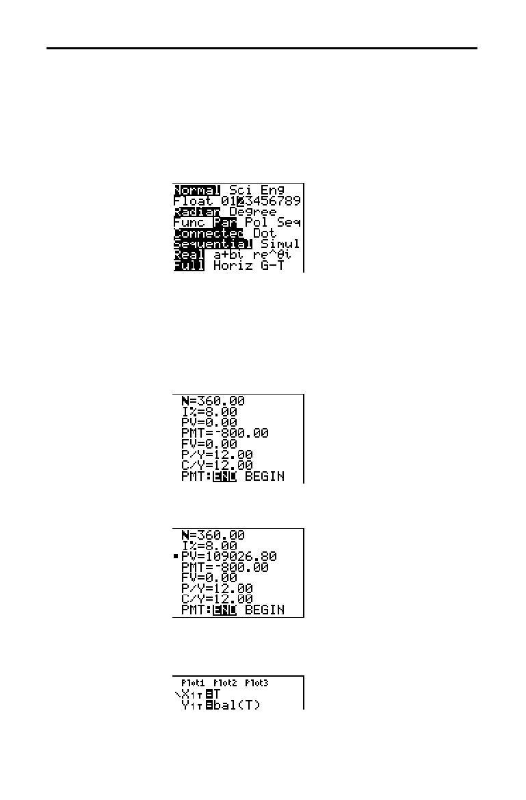
14-10 Financial Functions
8314FINA.DOC TI-83 international English Bob Fedorisko Revised: 02/19/01 12:50 PM Printed: 02/19/01 1:38 PM
Page 10 of 14
You want to buy a home with a 30-year mortgage at 8
percent APR. Monthly payments are 800. Calculate the
outstanding loan balance after each payment and display
the results in a graph and in the table.
1. Press
z
. Press
†
~
~
~
Í
to set the
fixed-decimal mode setting to
2. Press
†
†
~
Í
to
select
Par graphing mode.
2. Press
y
[
FINANCE
]
Í
to display the
TVM Solver
.
3. Press
360 to enter number of payments. Press
†
8 to
enter the interest rate. Press
†
†
Ì
800 to enter the
payment amount. Press
†
0 to enter the future value of
the mortgage. Press
†
12 to enter the payments per
year, which also sets the compounding periods per year
to
12. Press
†
†
Í
to select PMT:END.
4. Press
}
}
}
}
}
to place the cursor on the PV prompt.
Press
ƒ
[
SOLVE
] to solve for the present value.
5. Press
o
to display the parametric
Y=
editor. Turn off all
stat plots. Press
„
to define
X
1T
as T. Press
†
y
[
FINANCE
] 9
„¤
to define Y
1T
as bal(T).
Amortization
Example:
Calculating an
Outstanding
Loan Balance
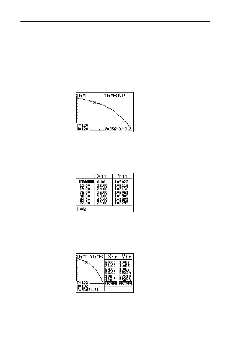
Financial Functions 14-11
8314FINA.DOC TI-83 international English Bob Fedorisko Revised: 02/19/01 12:50 PM Printed: 02/19/01 1:38 PM
Page 11 of 14
6. Press
p
to display the window variables. Enter
the values below.
Tmin=0 Xmin=0 Ymin=0
Tmax=360 Xmax=360 Ymax=125000
Tstep=12 Xscl=50 Yscl=10000
7. Press
r
to draw the graph and activate the trace
cursor. Press
~
and
|
to explore the graph of the
outstanding balance over time. Press a number and then
press
Í
to view the balance at a specific time
T.
8. Press
y
[
TBLSET
] and enter the values below.
TblStart=0
@
Tbl=12
9. Press
y
[
TABLE
] to display the table of outstanding
balances (
Y
1T
).
10.Press
z
†
†
†
†
†
†
†
~
~
Í
to select G
.
T
split-screen mode, in which the graph and table are
displayed simultaneously.
Press
r
to display
X
1T
(time) and Y
1T
(balance) in
the table.
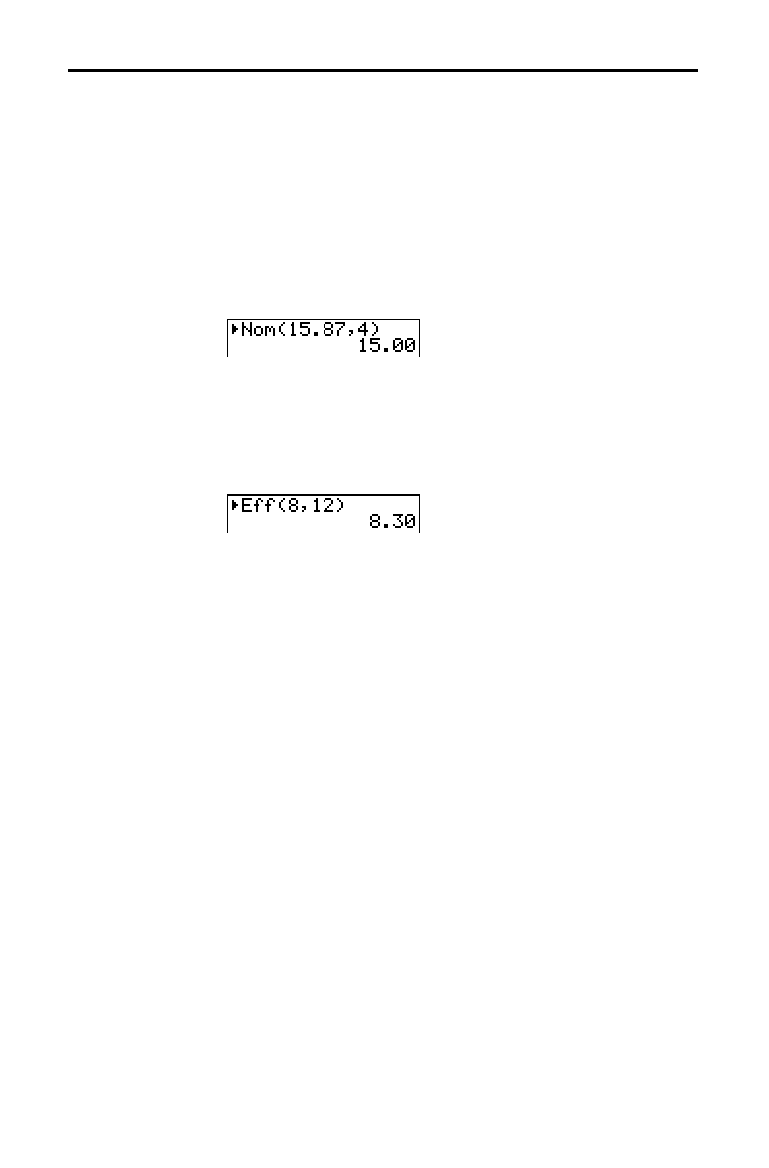
14-12 Financial Functions
8314FINA.DOC TI-83 international English Bob Fedorisko Revised: 02/19/01 12:50 PM Printed: 02/19/01 1:38 PM
Page 12 of 14
Use the interest conversion functions (menu items B and
C) to convert interest rates from an annual effective rate to
a nominal rate (
4
Nom(
) or from a nominal rate to an annual
effective rate (
4
Eff(
).
4
Nom(
computes the nominal interest rate.
effective rate
and
compounding periods
must be real numbers.
compounding periods
must be >0.
4
Nom(
effective rate
,
compounding periods
)
4
Eff(
computes the effective interest rate.
nominal rate
and
compounding periods
must be real numbers.
compounding periods
must be >0.
4
Eff(
nominal rate
,
compounding periods
)
Calculating Interest Conversion
Calculating an
Interest
Conversion
4
Nom(
4
Eff(
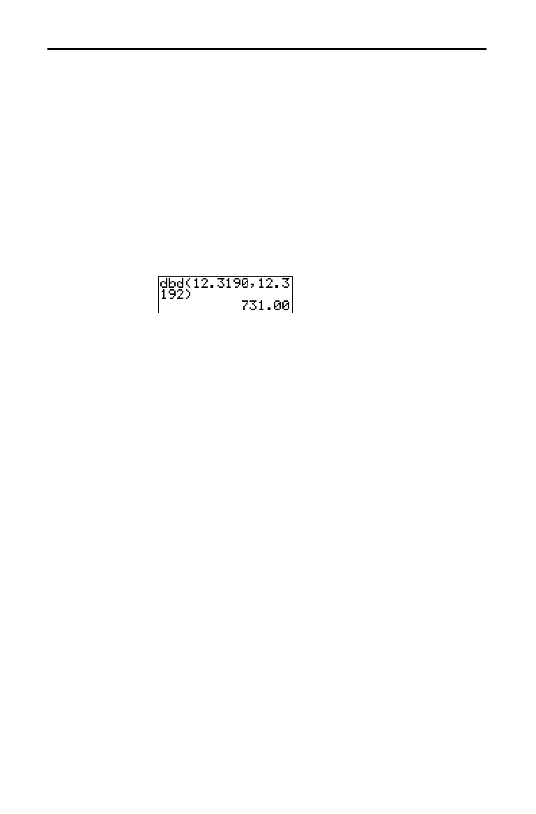
Financial Functions 14-13
8314FINA.DOC TI-83 international English Bob Fedorisko Revised: 02/19/01 12:50 PM Printed: 02/19/01 1:38 PM
Page 13 of 14
Use the date function dbd( (menu item D) to calculate the
number of days between two dates using the actual-day-
count method.
date1
and
date2
can be numbers or lists of
numbers within the range of the dates on the standard
calendar.
Note:
Dates must be between the years 1950 through 2049.
dbd(
date1
,
date2
)
You can enter
date1
and
date2
in either of two formats.
•
MM.DDYY (United States)
•
DDMM.YY (Europe)
The decimal placement differentiates the date formats.
Pmt_End and Pmt_Bgn (menu items E and F) specify a
transaction as an ordinary annuity or an annuity due. When
you execute either command, the
TVM Solver
is updated.
Pmt_End (payment end) specifies an ordinary annuity,
where payments occur at the end of each payment period.
Most loans are in this category.
Pmt_End is the default.
Pmt_End
On the
TVM Solver
’s PMT:END BEGIN line, select END to set
PMT to ordinary annuity.
Pmt_Bgn (payment beginning) specifies an annuity due,
where payments occur at the beginning of each payment
period. Most leases are in this category.
Pmt_Bgn
On the
TVM Solver
’s PMT:END BEGIN line, select BEGIN to
set
PMT to annuity due.
Finding Days between Dates/Defining Payment Method
dbd(
Defining the
Payment Method
Pmt_End
Pmt_Bgn

14-14 Financial Functions
8314FINA.DOC TI-83 international English Bob Fedorisko Revised: 02/19/01 12:50 PM Printed: 02/19/01 1:38 PM
Page 14 of 14
To display the
FINANCE VARS
menu, press
y
[
FINANCE
]
~
. You can use
TVM
variables in
TVM
functions and store
values to them on the home screen.
CALC VARS
1:
Ú
Total number of payment periods
2:
æ
Annual interest rate
3: PV
Present value
4: PMT
Payment amount
5: FV
Future value
6: P/Y
Number of payment periods per year
7: C/Y
Number of compounding periods/year
Ú
,
æ
, PV, PMT, and FV are the five
TVM
variables. They
represent the elements of common financial transactions,
as described in the table above.
æ
is an annual interest rate
that is converted to a per-period rate based on the values
of
P/Y and C/Y.
P/Y is the number of payment periods per year in a
financial transaction.
C/Y is the number of compounding periods per year in the
same transaction.
When you store a value to
P/Y, the value for C/Y
automatically changes to the same value. To store a unique
value to
C/Y, you must store the value to C/Y after you have
stored a value to
P/Y.
Using the TVM Variables
FINANCE VARS
Menu
Ú
,
æ
, PV, PMT,
FV
P/Y and C/Y
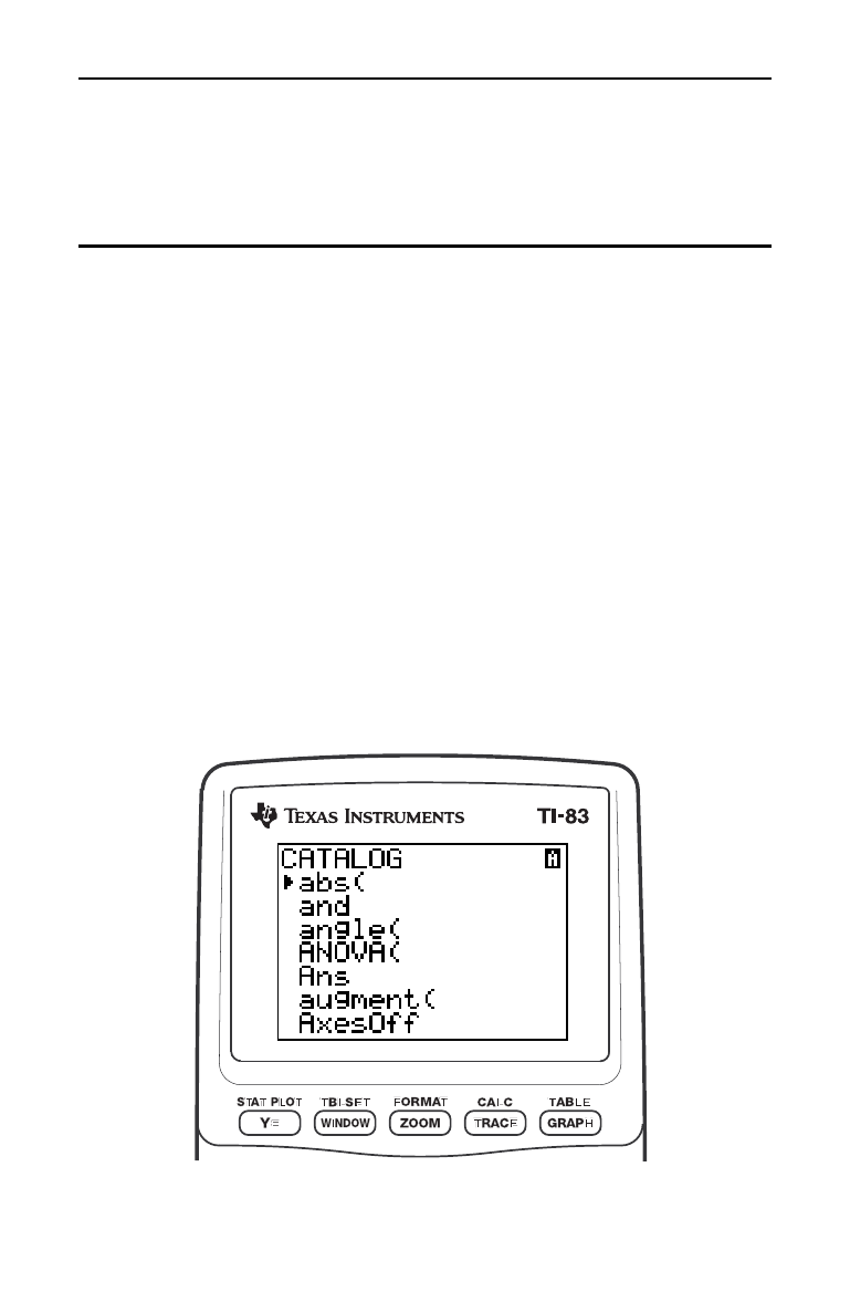
CATALOG, Strings, Hyperbolic Functions 15-1
8315CATS.DOC TI-83 international English Bob Fedorisko Revised: 02/19/01 12:54 PM Printed: 02/19/01 1:39
PM Page 1 of 10
15
CATALOG, Strin
g
s,
H
y
perbolic Functions
Browsing the TI
-
83
CATALOG
...........................
15-2
Entering and Using Strings
...............................
15-3
Storing Strings to String Variables
.......................
15-4
String Functions and Instructions in the
CATALOG
......
15-6
Hyperbolic Functions in the
CATALOG
..................
15-10
Contents
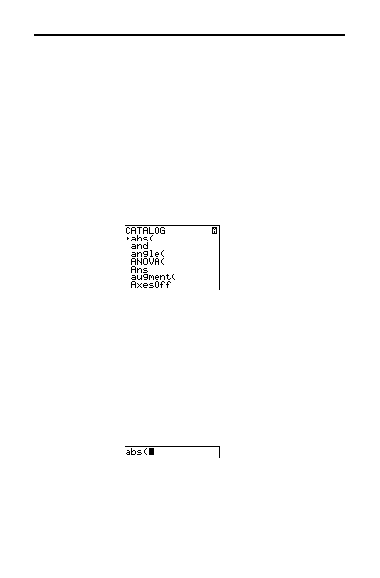
15-2 CATALOG, Strings, Hyperbolic Functions
8315CATS.DOC TI-83 international English Bob Fedorisko Revised: 02/19/01 12:54 PM Printed: 02/19/01 1:39
PM Page 2 of 10
The
CATALOG
is an alphabetical list of all functions and
instructions on the TI
-
83. You also can access each
CATALOG
item from a menu or the keyboard, except:
•
The six string functions (page 15
.
6)
•
The six hyperbolic functions (page 15
.
10)
•
The
solve( instruction without the equation solver editor
(Chapter 2)
•
The inferential stat functions without the inferential stat
editors (Chapter 13)
Note:
The only
CATALOG
programming commands you can execute
from the home screen are
GetCalc(
,
Get(
, and
Send(
.
To select a
CATALOG
item, follow these steps.
1. Press
y
ã
CATALOGä
to display the
CATALOG
.
The
4
in the first column is the selection cursor.
2. Press
†
or
}
to scroll the
CATALOG
until the selection
cursor points to the item you want.
•
To jump to the first item beginning with a particular
letter, press that letter; alpha-lock is on.
•
Items that begin with a number are in alphabetical
order according to the first letter after the number.
For example,
2
.
PropZTest( is among the items that
begin with the letter P.
•
Functions that appear as symbols, such as
+,
L
1
, <,
and
‡
(
, follow the last item that begins with Z. To
jump to the first symbol, !, press [
q
].
3. Press
Í
to paste the item to the current screen.
Tip:
From the top of the
CATALOG
menu, press
}
to move to the
bottom. From the bottom, press
†
to move to the top.
Browsing the TI-83 CATALOG
What Is the
CATALOG?
Selecting an Item
from the
CATALOG
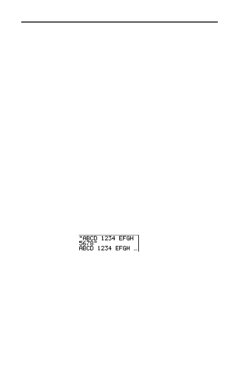
CATALOG, Strings, Hyperbolic Functions 15-3
8315CATS.DOC TI-83 international English Bob Fedorisko Revised: 02/19/01 12:54 PM Printed: 02/19/01 1:39
PM Page 3 of 10
A string is a sequence of characters that you enclose within
quotation marks. On the TI
-
83, a string has two primary
applications.
•
It defines text to be displayed in a program.
•
It accepts input from the keyboard in a program.
Characters are the units that you combine to form a string.
•
Count each number, letter, and space as one character.
•
Count each instruction or function name, such as
sin( or
cos(, as one character; the TI
-
83 interprets each
instruction or function name as one character.
To enter a string on a blank line on the home screen or in a
program, follow these steps.
1. Press
ƒ
[
ã
] to indicate the beginning of the string.
2. Enter the characters that comprise the string.
•
Use any combination of numbers, letters, function
names, or instruction names to create the string.
•
To enter a blank space, press
ƒ
[
'
].
•
To enter several alpha characters in a row, press
y
[
A
.
LOCK
] to activate alpha-lock.
3. Press
ƒ
[
ã
] to indicate the end of the string.
"
string
"
4. Press
Í
. On the home screen, the string is displayed
on the next line without quotations. An ellipsis (
...)
indicates that the string continues beyond the screen.
To scroll the entire string, press
~
and
|
.
Note:
Quotation marks do not count as string characters.
Entering and Using Strings
What Is a String?
Entering a String
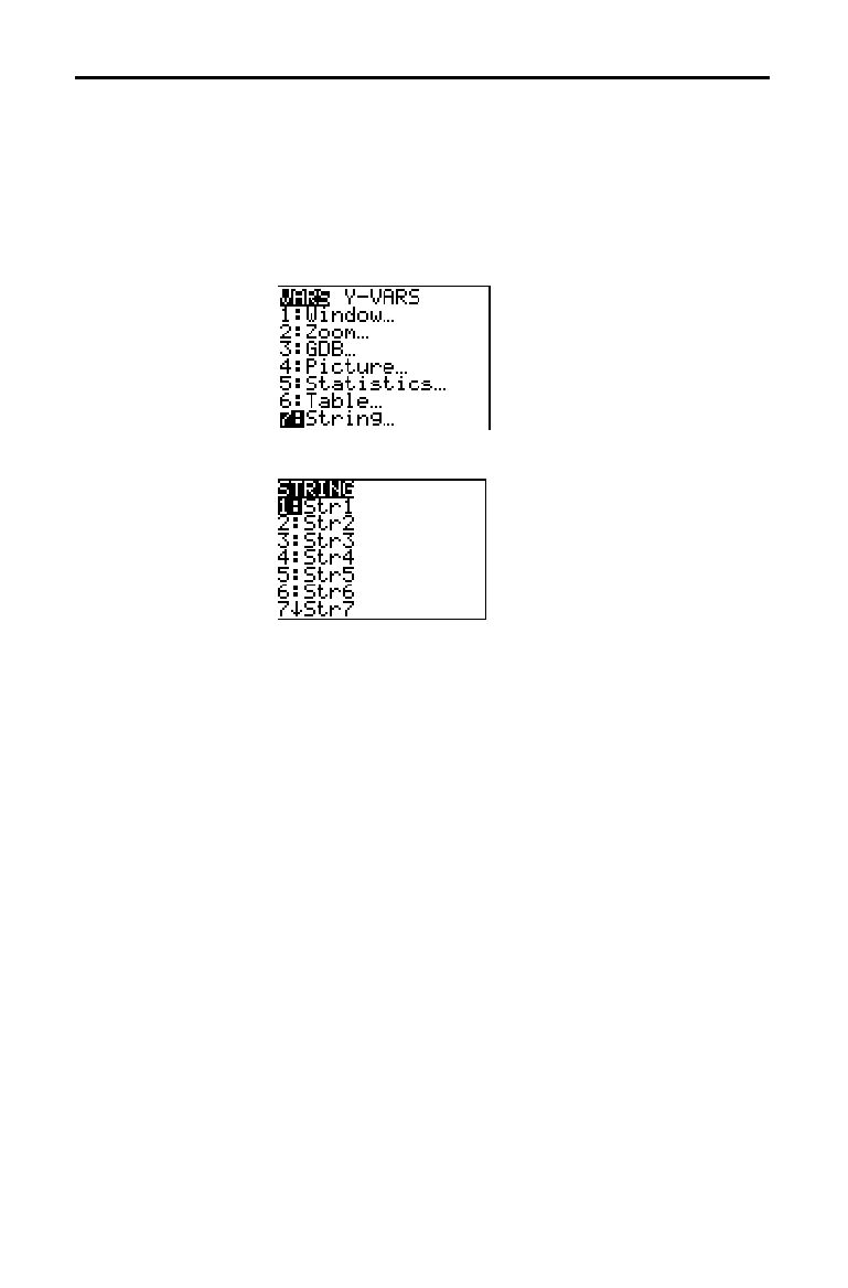
15-4 CATALOG, Strings, Hyperbolic Functions
8315CATS.DOC TI-83 international English Bob Fedorisko Revised: 02/19/01 12:54 PM Printed: 02/19/01 1:39
PM Page 4 of 10
The TI
-
83 has 10 variables to which you can store strings.
You can use string variables with string functions and
instructions.
To display the
VARS STRING
menu, follow these steps.
1. Press
to display the
VARS
menu. Move the cursor
to
7:String.
2. Press
Í
to display the
STRING
secondary menu.
Storing Strings to String Variables
String Variables
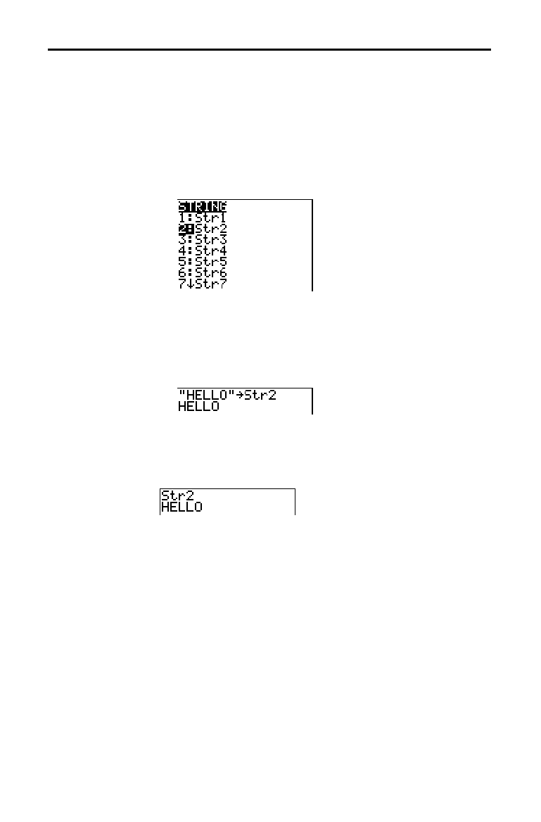
CATALOG, Strings, Hyperbolic Functions 15-5
8315CATS.DOC TI-83 international English Bob Fedorisko Revised: 02/19/01 12:54 PM Printed: 02/19/01 1:39
PM Page 5 of 10
To store a string to a string variable, follow these steps.
1. Press
ƒ
[
ã
], enter the string, and press
ƒ
[
ã
].
2. Press
¿
.
3. Press
7 to display the
VARS STRING
menu.
4. Select the string variable (from
Str1 to Str9, or Str0) to
which you want to store the string.
The string variable is pasted to the current cursor
location, next to the store symbol (
!
).
5. Press
Í
to store the string to the string variable. On
the home screen, the stored string is displayed on the
next line without quotation marks.
To display the contents of a string variable on the home
screen, select the string variable from the
VARS STRING
menu, and then press
Í
. The string is displayed.
Storing a String
to a String
Variable
Displaying the
Contents of a
String Variable

15-6 CATALOG, Strings, Hyperbolic Functions
8315CATS.DOC TI-83 international English Bob Fedorisko Revised: 02/19/01 12:54 PM Printed: 02/19/01 1:39
PM Page 6 of 10
String functions and instructions are available only from
the
CATALOG
. The table below lists the string functions
and instructions in the order in which they appear among
the other
CATALOG
menu items. The ellipses in the table
indicate the presence of additional
CATALOG
items.
CATALOG
...
Equ
4
String(
Converts an equation to a string.
expr(
Converts a string to an expression.
...
inString(
Returns a character’s place number.
...
length(
Returns a string’s character length.
...
String
4
Equ(
Converts a string to an equation.
sub(
Returns a string subset as a string.
...
To concatenate two or more strings, follow these steps.
1. Enter
string1
, which can be a string or string name.
2. Press
Ã
.
3. Enter
string2
, which can be a string or string name. If
necessary, press
Ã
and enter
string3
, and so on.
string1
+
string2
+
string3
. . .
4. Press
Í
to display the strings as a single string.
To select a string function or instruction and paste it to the
current screen, follow the steps on page 15
.
2.
String Functions and Instructions in the CATALOG
Displaying String
Functions and
Instructions in
the CATALOG
+ (Concatenation)
Selecting a String
Function from
the CATALOG
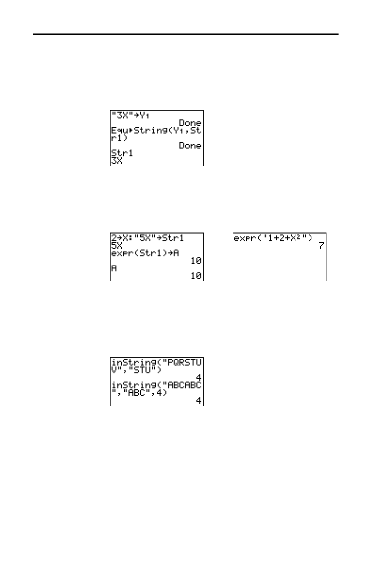
CATALOG, Strings, Hyperbolic Functions 15-7
8315CATS.DOC TI-83 international English Bob Fedorisko Revised: 02/19/01 12:54 PM Printed: 02/19/01 1:39
PM Page 7 of 10
Equ
4
String( converts to a string an equation that is stored
to any
VARS Y
.
VARS
variable. Y
n
contains the equation.
Str
n
(from
Str1 to Str9, or Str0) is the string variable to
which you want the equation to be stored as a string.
Equ
4
String(Y
n
,Str
n
)
expr( converts the character string contained in
string
to
an expression and executes it.
string
can be a string or a
string variable.
expr(
string
)
inString( returns the character position in
string
of the first
character of
substring
.
string
can be a string or a string
variable.
start
is an optional character position at which to
start the search; the default is 1.
inString(
string
,
substring
[
,
start
]
)
Note:
If
string
does not contain
substring
, or
start
is greater than the
length of
string
,
inString(
returns
0
.
Equ
4
String(
expr(
inString(
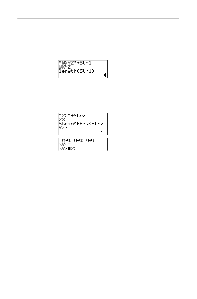
15-8 CATALOG, Strings, Hyperbolic Functions
8315CATS.DOC TI-83 international English Bob Fedorisko Revised: 02/19/01 12:54 PM Printed: 02/19/01 1:39
PM Page 8 of 10
length( returns the number of characters in
string
.
string
can be a string or string variable.
Note:
An instruction or function name, such as
sin(
or
cos(
,
counts as
one character.
length(
string
)
String
4
Equ( converts
string
into an equation and stores the
equation to
Y
n
.
string
can be a string or string variable.
String
4
Equ( is the inverse of Equ
4
String(.
String
4
Equ(
string
,Y
n
)
length(
String
4
Equ(
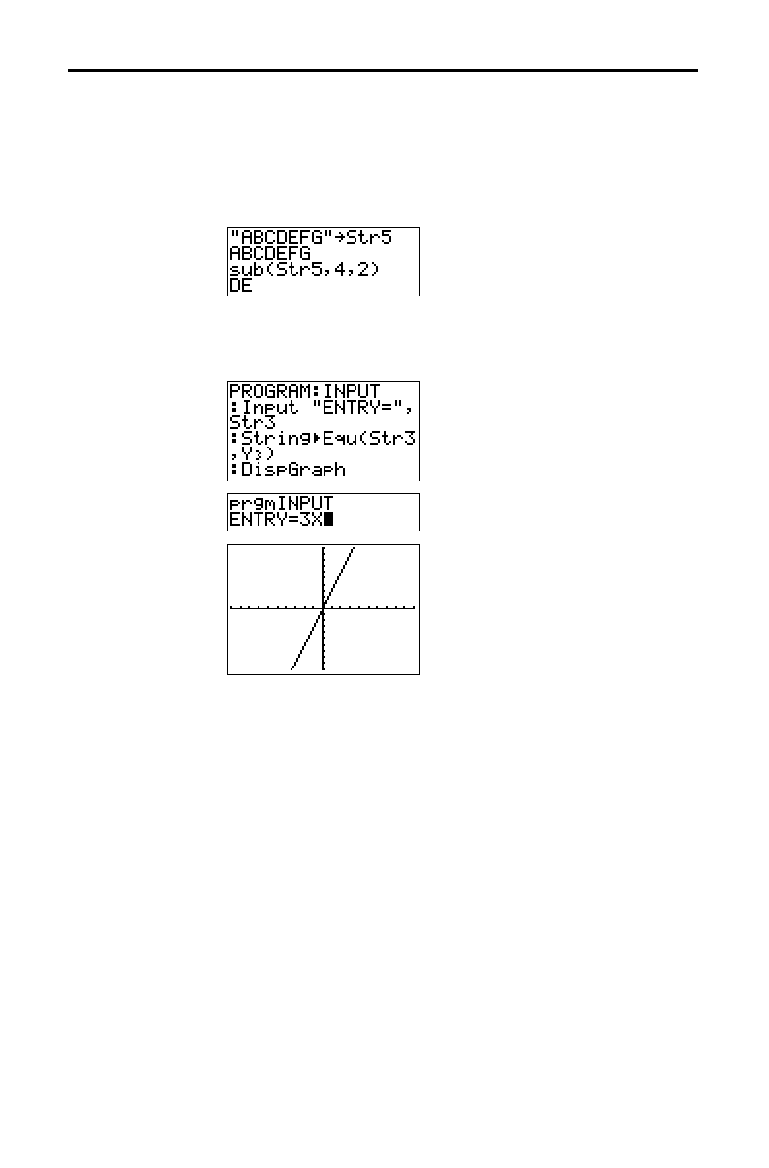
CATALOG, Strings, Hyperbolic Functions 15-9
8315CATS.DOC TI-83 international English Bob Fedorisko Revised: 02/19/01 12:54 PM Printed: 02/19/01 1:39
PM Page 9 of 10
sub( returns a string that is a subset of an existing
string
.
string
can be a string or a string variable.
begin
is the
position number of the first character of the subset.
length
is the number of characters in the subset.
sub(
string
,
begin
,
length
)
In a program, you can enter a function to graph during
program execution using these commands.
Note:
When you execute this program, enter a function to store to
Y3
at the
ENTRY=
prompt.
sub(
Entering a
Function to
Graph during
Program
Execution
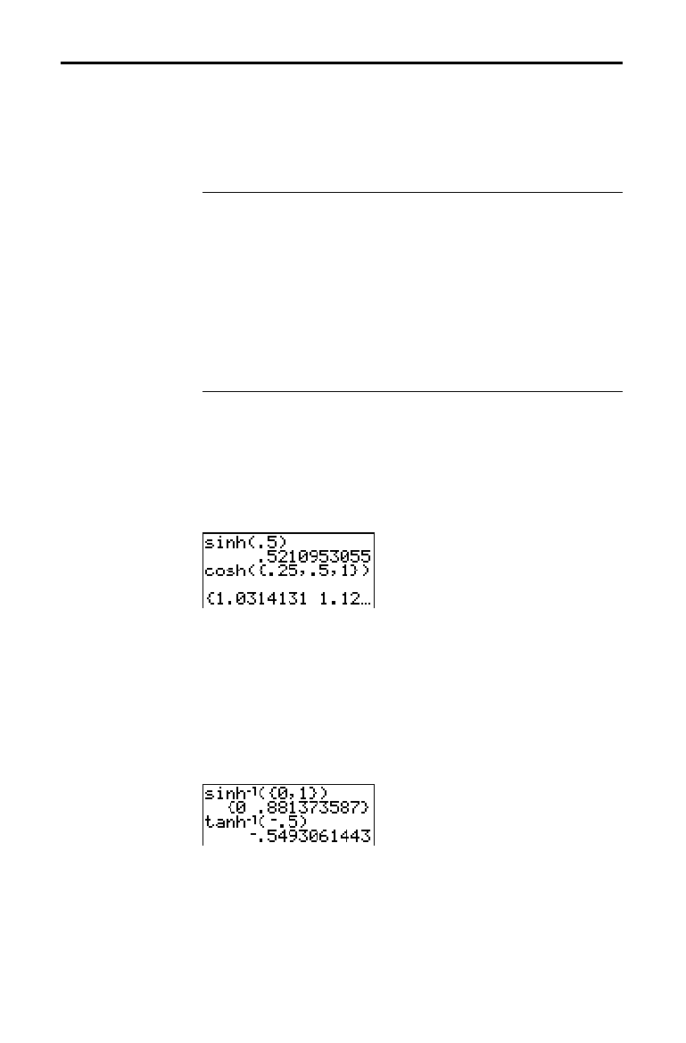
15-10 CATALOG, Strings, Hyperbolic Functions
8315CATS.DOC TI-83 international English Bob Fedorisko Revised: 02/19/01 12:54 PM Printed: 02/19/01 1:39
PM Page 10 of 10
The hyperbolic functions are available only from the
CATALOG
. The table below lists the hyperbolic functions in
the order in which they appear among the other
CATALOG
menu items. The ellipses in the table indicate the presence
of additional
CATALOG
items.
CATALOG
...
cosh(
Hyperbolic cosine
cosh
L
1
(
Hyperbolic arccosine
...
sinh(
Hyperbolic sine
sinh
L
1
(
Hyperbolic arcsine
...
tanh(
Hyperbolic tangent
tanh
L
1
(
Hyperbolic arctangent
...
sinh(, cosh(, and tanh( are the hyperbolic functions. Each is
valid for real numbers, expressions, and lists.
sinh(
value
)
cosh(
value
)
tanh(
value
)
sinh
L
1
( is the hyperbolic arcsine function. cosh
L
1
( is the
hyperbolic arccosine function.
tanh
L
1
( is the hyperbolic
arctangent function. Each is valid for real numbers,
expressions, and lists.
sinh
L
1
(
value
)
cosh
L
1
(
value
)
sinh
L
1
(
value
)
Hyperbolic Functions in the CATALOG
Hyperbolic
Functions
sinh(, cosh(,
tanh(
sinh
L
1
(, cosh
L
1
(,
tanh
L
1
(
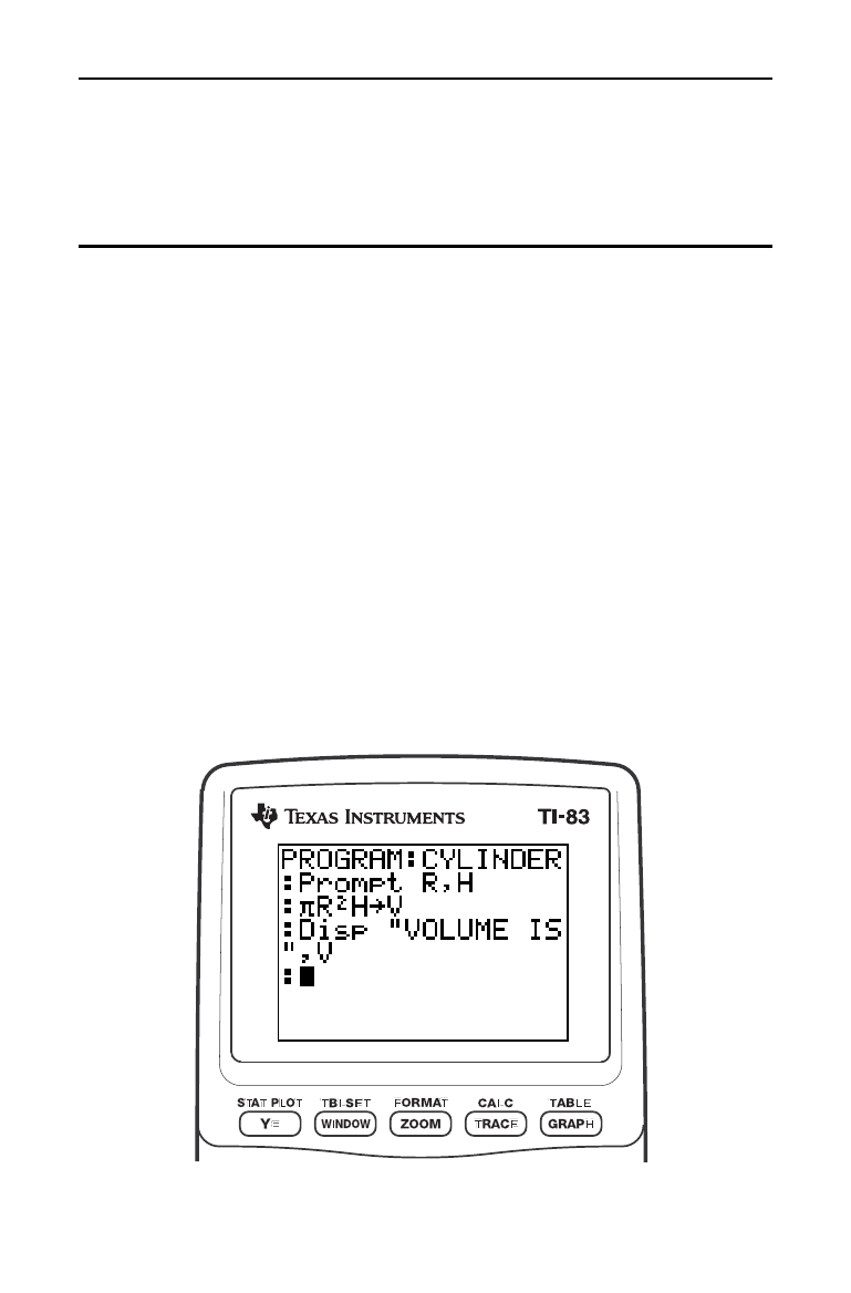
Programming 16-1
8316PROG.DOC TI-83 international English Bob Fedorisko Revised: 02/19/01 1:23 PM Printed: 02/19/01 1:39
PM Page 1 of 22
16
Pro
g
rammin
g
Getting Started: Volume of a Cylinder
....................
16-2
Creating and Deleting Programs
.........................
16-4
Entering Command Lines and Executing Programs
......
16-5
Editing Programs
........................................
16-6
Copying and Renaming Programs
........................
16-7
PRGM CTL
(Control) Instructions
.......................
16-8
PRGM I/O
(Input/Output) Instructions
...................
16-16
Calling Other Programs as Subroutines
..................
16-22
Contents
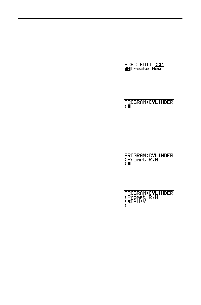
16-2 Programming
8316PROG.DOC TI-83 international English Bob Fedorisko Revised: 02/19/01 1:23 PM Printed: 02/19/01 1:39
PM Page 2 of 22
Getting Started is a fast-paced introduction. Read the chapter for details.
A program is a set of commands that the TI
-
83 executes sequentially, as if you
had entered them from the keyboard. Create a program that prompts for the
radius R and the height H of a cylinder and then computes its volume.
1. Press
~
~
to display the
PRGM NEW
menu.
2. Press
Í
to select 1:Create New. The
Name= prompt is displayed, and alpha-lock
is on. Press [
C
] [
Y
] [
L
] [
I
] [
N
] [
D
] [
E
] [
R
], and
then press
Í
to name the program
CYLINDER.
You are now in the program editor. The
colon (
: ) in the first column of the second
line indicates the beginning of a command
line.
3. Press
~
2 to select 2:Prompt from
the
PRGM I/O
menu. Prompt is copied to
the command line. Press
ƒ
[
R
]
¢
ƒ
[
H
] to enter the variable names for
radius and height. Press
Í
.
4. Press
y
ãpä
ƒ
[
R
]
¡
ƒ
[
H
]
¿
ƒ
[
V
]
Í
to enter the expression
p
R
2
H and store it to the variable V.
Getting Started: Volume of a Cylinder
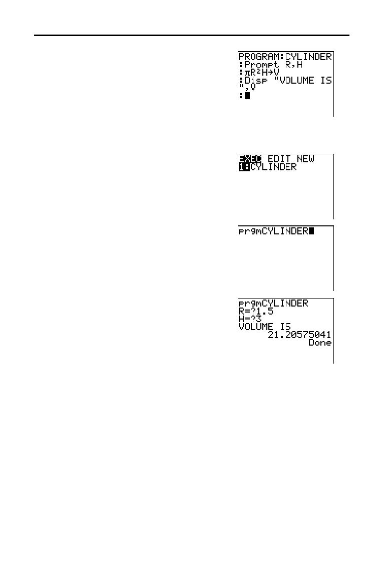
Programming 16-3
8316PROG.DOC TI-83 international English Bob Fedorisko Revised: 02/19/01 1:23 PM Printed: 02/19/01 1:39
PM Page 3 of 22
5. Press
~
3 to select 3:Disp from the
PRGM I/O
menu. Disp is pasted to the
command line. Press
y
[
A.LOCK
]
ããä
[
V
]
[
O
] [
L
] [
U
] [
M
] [
E
][
'
] [
I
] [
S
]
ããä
ƒ
¢
ƒ
[
V
]
Í
to set up the program to
display the text
VOLUME IS on one line and
the calculated value of
V on the next.
6. Press
y
[
QUIT
] to display the home
screen.
7. Press
to display the
PRGM EXEC
menu. The items on this menu are the
names of stored programs.
8. Press
Í
to paste prgmCYLINDER to the
current cursor location. (If
CYLINDER is
not item
1 on your
PRGM EXEC
menu,
move the cursor to
CYLINDER before you
press
Í
.)
9. Press
Í
to execute the program. Enter
1.5 for the radius, and then press
Í
.
Enter
3 for the height, and then press
Í
. The text
VOLUME IS, the value of V,
and
Done are displayed.
Repeat steps 7 through 9 and enter
different values for
R and H.
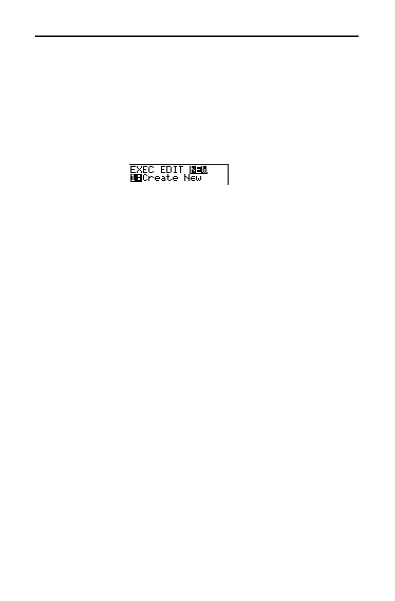
16-4 Programming
8316PROG.DOC TI-83 international English Bob Fedorisko Revised: 02/19/01 1:23 PM Printed: 02/19/01 1:39
PM Page 4 of 22
A program is a set of one or more command lines. Each
line contains one or more instructions. When you execute a
program, the TI
-
83 performs each instruction on each
command line in the same order in which you entered
them. The number and size of programs that the TI
-
83 can
store is limited only by available memory.
To create a new program, follow these steps.
1. Press
|
to display the
PRGM NEW
menu.
2. Press
Í
to select 1:Create New. The Name= prompt
is displayed, and alpha-lock is on.
3. Press a letter from A to Z or
q
to enter the first
character of the new program name.
Note:
A program name can be one to eight characters long. The
first character must be a letter from A to Z or
q
. The second
through eighth characters can be letters, numbers, or
q
.
4. Enter zero to seven letters, numbers, or
q
to complete
the new program name.
5. Press
Í
. The program editor is displayed.
6. Enter one or more program commands (page 16
.
5).
7. Press
y
[
QUIT
] to leave the program editor and return
to the home screen.
To check whether adequate memory is available for a
program you want to enter, press
y
[
MEM
], and then
select
1:Check RAM from the
MEMORY
menu (Chapter 18).
To increase available memory, press
y
[
MEM
], and then
select
2:Delete from the
MEMORY
menu (Chapter 18).
To delete a specific program, press
y
[
MEM
], select
2:Delete from the
MEMORY
menu, and then select 7:Prgm
from the
DELETE FROM
secondary menu (Chapter 18).
Creating and Deleting Programs
What Is a
Program?
Creating a New
Program
Managing
Memory and
Deleting a
Program

Programming 16-5
8316PROG.DOC TI-83 international English Bob Fedorisko Revised: 02/19/01 1:23 PM Printed: 02/19/01 1:39
PM Page 5 of 22
You can enter on a command line any instruction or
expression that you could execute from the home screen. In
the program editor, each new command line begins with a
colon. To enter more than one instruction or expression on a
single command line, separate each with a colon.
Note:
A command line can be longer than the screen is wide; long
command lines wrap to the next screen line.
While in the program editor, you can display and select
from menus. You can return to the program editor from a
menu in either of two ways.
•
Select a menu item, which pastes the item to the
current command line.
•
Press
‘
.
When you complete a command line, press
Í
. The
cursor moves to the next command line.
Programs can access variables, lists, matrices, and strings
saved in memory. If a program stores a new value to a
variable, list, matrix, or string, the program changes the
value in memory during execution.
You can call another program as a subroutine (page 16
.
15
and page 16
.
22).
To execute a program, begin on a blank line on the home
screen and follow these steps.
1. Press
to display the
PRGM EXEC
menu.
2. Select a program name from the
PRGM EXEC
menu
(page 16
.
7).
prgm
name
is pasted to the home screen
(for example,
prgmCYLINDER).
3. Press
Í
to execute the program. While the program
is executing, the busy indicator is on.
Last Answer (
Ans) is updated during program execution.
Last Entry is not updated as each command is executed
(Chapter 1).
The TI
-
83 checks for errors during program execution. It
does not check for errors as you enter a program.
To stop program execution, press
É
. The
ERR:BREAK
menu is displayed.
•
To return to the home screen, select
1:Quit.
•
To go where the interruption occurred, select
2:Goto.
Entering Command Lines and Executing Programs
Entering a
Program
Command Line
Executing a
Program
Breaking a
Program

16-6 Programming
8316PROG.DOC TI-83 international English Bob Fedorisko Revised: 02/19/01 1:23 PM Printed: 02/19/01 1:39
PM Page 6 of 22
To edit a stored program, follow these steps.
1. Press
~
to display the
PRGM EDIT
menu.
2. Select a program name from the
PRGM EDIT
menu (page
16
.
7). Up to the first seven lines of the program are
displayed.
Note:
The program editor does not display a
$
to indicate that
a program continues beyond the screen.
3. Edit the program command lines.
•
Move the cursor to the appropriate location, and
then delete, overwrite, or insert.
•
Press
‘
to clear all program commands on the
command line (the leading colon remains), and then
enter a new program command.
Tip:
To move the cursor to the beginning of a command line, press
y
|
; to move to the end, press
y
~
. To scroll the cursor down
seven command lines, press
ƒ
†
. To scroll the cursor up seven
command lines, press
ƒ
}
.
To insert a new command line anywhere in the program,
place the cursor where you want the new line, press
y
[
INS
], and then press
Í
. A colon indicates a new line.
To delete a command line, place the cursor on the line,
press
‘
to clear all instructions and expressions on
the line, and then press
{
to delete the command line,
including the colon.
Editing Programs
Editing a
Program
Inserting and
Deleting
Command Lines

Programming 16-7
8316PROG.DOC TI-83 international English Bob Fedorisko Revised: 02/19/01 1:23 PM Printed: 02/19/01 1:39
PM Page 7 of 22
To copy all command lines from one program into a new
program, follow steps 1 through 5 for Creating a New
Program (page 16
.
4), and then follow these steps.
1. Press
y
[
RCL
]. Rcl is displayed on the bottom line of
the program editor in the new program (Chapter 1).
2. Press
|
to display the
PRGM EXEC
menu.
3. Select a name from the menu.
prgm
name
is pasted to
the bottom line of the program editor.
4. Press
Í
. All command lines from the selected
program are copied into the new program.
Copying programs has at least two convenient
applications.
•
You can create a template for groups of instructions
that you use frequently.
•
You can rename a program by copying its contents into
a new program.
Note:
You also can copy all the command lines from one existing
program to another existing program using
RCL
.
The TI
-
83 sorts
PRGM EXEC
and
PRGM EDIT
menu items
automatically into alphanumerical order. Each menu only
labels the first 10 items using
1 through 9, then 0.
To jump to the first program name that begins with a
particular alpha character or
q
, press
ƒ
[
letter from A
to Z or
q
].
Tip:
From the top of either the
PRGM EXEC
or
PRGM EDIT
menu,
press
}
to move to the bottom. From the bottom, press
†
to move to
the top. To scroll the cursor down the menu seven items, press
ƒ
†
. To scroll the cursor up the menu seven items, press
ƒ
}
.
Copying and Renaming Programs
Copying and
Renaming a
Program
Scrolling the
PRGM EXEC and
PRGM EDIT
Menus

16-8 Programming
8316PROG.DOC TI-83 international English Bob Fedorisko Revised: 02/19/01 1:23 PM Printed: 02/19/01 1:39
PM Page 8 of 22
To display the
PRGM CTL
(program control) menu, press
from the program editor only.
CTL I/O EXEC
1: If
Creates a conditional test.
2: Then
Executes commands when If is true.
3: Else
Executes commands when If is false.
4: For(
Creates an incrementing loop.
5: While
Creates a conditional loop.
6: Repeat
Creates a conditional loop.
7: End
Signifies the end of a block.
8: Pause
Pauses program execution.
9: Lbl
Defines a label.
0: Goto
Goes to a label.
A: IS>(
Increments and skips if greater than.
B: DS<(
Decrements and skips if less than.
C: Menu(
Defines menu items and branches.
D: prgm
Executes a program as a subroutine.
E: Return
Returns from a subroutine.
F: Stop
Stops execution.
G: DelVar
Deletes a variable from within program.
H: GraphStyle(
Designates the graph style to be drawn.
These menu items direct the flow of an executing program.
They make it easy to repeat or skip a group of commands
during program execution. When you select an item from
the menu, the name is pasted to the cursor location on a
command line in the program.
To return to the program editor without selecting an item,
press
‘
.
Program control instructions tell the TI
-
83 which
command to execute next in a program.
If, While, and
Repeat check a defined condition to determine which
command to execute next. Conditions frequently use
relational or Boolean tests (Chapter 2), as in:
If A<7:A+1
!
A
or
If N=1 and M=1:Goto Z
PRGM CTL (Control) Instructions
PRGM CTL Menu
Controlling
Program Flow
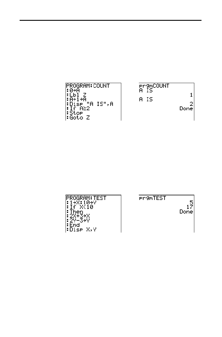
Programming 16-9
8316PROG.DOC TI-83 international English Bob Fedorisko Revised: 02/19/01 1:23 PM Printed: 02/19/01 1:39
PM Page 9 of 22
Use If for testing and branching. If
condition
is false (zero),
then the
command
immediately following
If is skipped. If
condition
is true (nonzero), then the next
command
is
executed.
If instructions can be nested.
:If
condition
:
command
(if true)
:
command
Program Output
Then following an If executes a group of
commands
if
condition
is true (nonzero).
End identifies the end of the
group of
commands
.
:If
condition
:Then
:
command
(if true)
:
command
(if true)
:End
:
command
Program Output
If
If
.
Then
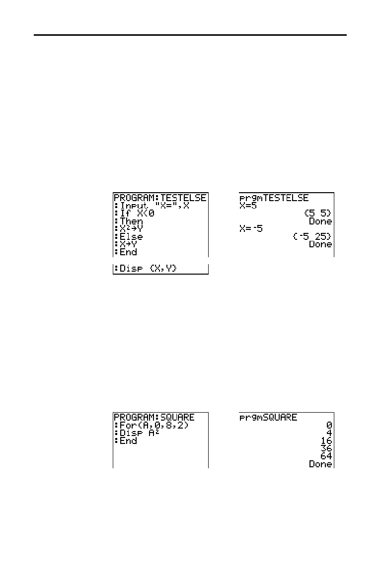
16-10 Programming
8316PROG.DOC TI-83 international English Bob Fedorisko Revised: 02/19/01 1:23 PM Printed: 02/19/01 1:39
PM Page 10 of 22
Else following If
.
Then executes a group of
commands
if
condition
is false (zero).
End identifies the end of the
group of
commands
.
:If
condition
:Then
:
command
(if true)
:
command
(if true)
:Else
:
command
(if false)
:
command
(if false)
:End
:
command
Program Output
For( loops and increments. It increments
variable
from
begin
to
end
by
increment
.
increment
is optional (default
is 1) and can be negative (
end
<
begin
).
end
is a maximum
or minimum value not to be exceeded.
End identifies the
end of the loop.
For( loops can be nested.
:For(
variable
,
begin
,
end
[
,
increment
]
)
:
command
(while
end
not exceeded)
:
command
(while
end
not exceeded)
:End
:
command
Program Output
If-Then-Else
For(
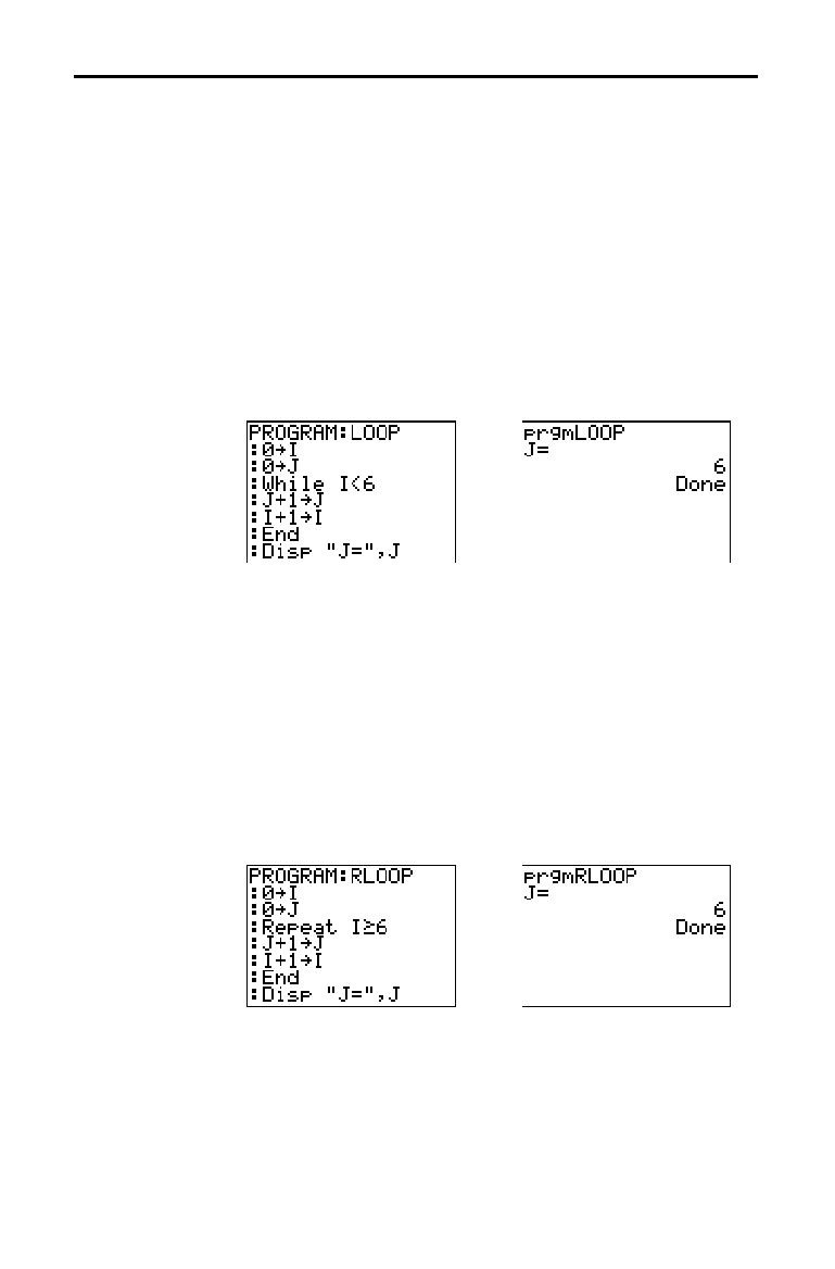
Programming 16-11
8316PROG.DOC TI-83 international English Bob Fedorisko Revised: 02/19/01 1:23 PM Printed: 02/19/01 1:39
PM Page 11 of 22
While performs a group of
commands
while
condition
is
true.
condition
is frequently a relational test (Chapter 2).
condition
is tested when
While is encountered. If
condition
is true (nonzero), the program executes a group
of
commands
.
End signifies the end of the group. When
condition
is false (zero), the program executes each
command
following
End. While instructions can be nested.
:While
condition
:
command
(while
condition
is true)
:
command
(while
condition
is true)
:End
:
command
Program Output
Repeat repeats a group of
commands
until
condition
is
true (nonzero). It is similar to
While, but
condition
is tested
when
End is encountered; therefore, the group of
commands
is always executed at least once.
Repeat
instructions can be nested.
:Repeat
condition
:
command
(until
condition
is true)
:
command
(until
condition
is true)
:End
:
c
ommand
Program Output
While
Repeat
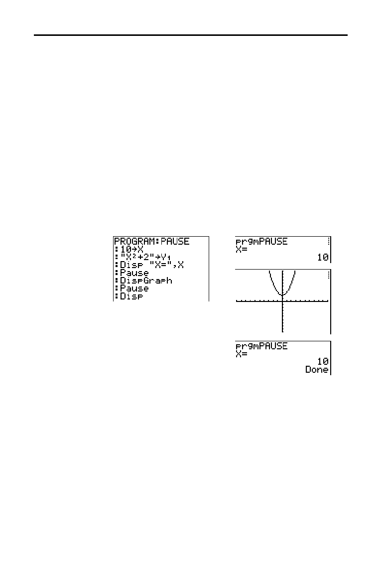
16-12 Programming
8316PROG.DOC TI-83 international English Bob Fedorisko Revised: 02/19/01 1:23 PM Printed: 02/19/01 1:39
PM Page 12 of 22
End identifies the end of a group of
commands
. You must
include an
End instruction at the end of each For(, While, or
Repeat loop. Also, you must paste an End instruction at the
end of each
If
.
Then group and each If
.
Then
.
Else group.
Pause suspends execution of the program so that you can
see answers or graphs. During the pause, the pause
indicator is on in the top-right corner. Press
Í
to
resume execution.
•
Pause without a
value
temporarily pauses the program.
If the DispGraph or Disp instruction has been executed,
the appropriate screen is displayed.
•
Pause with
value
displays
value
on the current home
screen.
value
can be scrolled.
Pause [
value
]
Program Output
End
Pause
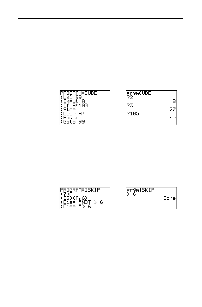
Programming 16-13
8316PROG.DOC TI-83 international English Bob Fedorisko Revised: 02/19/01 1:23 PM Printed: 02/19/01 1:39
PM Page 13 of 22
Lbl (label) and Goto (go to) are used together for
branching.
Lbl specifies the
label
for a command.
label
can be one or
two characters (
A through Z, 0 through 99, or
q
).
Lbl
label
Goto causes the program to branch to
label
when Goto is
encountered.
Goto
label
Program Output
IS>( (increment and skip) adds 1 to
variable.
If the answer
is >
value
(which can be an expression), the next
command
is skipped; if the answer is
{
value
, the next
command
is executed.
variable
cannot be a system
variable.
:IS>(
variable
,
value
)
:
command
(if answer
value
)
:
command
(if answer >
value
)
Program Output
Note:
IS>(
is not a looping instruction.
Lbl, Goto
IS>(
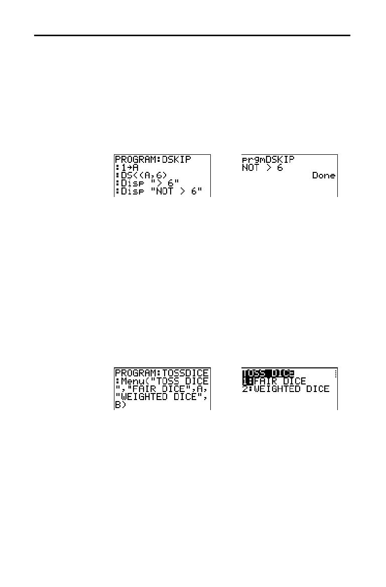
16-14 Programming
8316PROG.DOC TI-83 international English Bob Fedorisko Revised: 02/19/01 1:23 PM Printed: 02/19/01 1:39
PM Page 14 of 22
DS<( (decrement and skip) subtracts 1 from
variable
. If the
answer is <
value
(which can be an expression), the next
command
is skipped; if the answer is
|
value
, the next
command
is executed.
variable
cannot be a system
variable.
:DS<(variable,value)
:
command
(if answer
‚
value
)
:
command
(if answer <
value
)
Program Output
Note:
DS<(
is not a looping instruction.
Menu( sets up branching within a program. If Menu( is
encountered during program execution, the menu screen is
displayed with the specified menu items, the pause
indicator is on, and execution pauses until you select a
menu item.
The menu
title
is enclosed in quotation marks (
" ). Up to
seven pairs of menu items follow. Each pair comprises a
text
item (also enclosed in quotation marks) to be
displayed as a menu selection, and a
label
item to which to
branch if you select the corresponding menu selection.
Menu("
title
","
text1
",
label1
,"
text2
",
label2
, . . .)
Program Output
The program above pauses until you select 1 or 2. If you
select
2, for example, the menu disappears and the
program continues execution at
Lbl B.
DS<(
Menu(

Programming 16-15
8316PROG.DOC TI-83 international English Bob Fedorisko Revised: 02/19/01 1:23 PM Printed: 02/19/01 1:39
PM Page 15 of 22
Use prgm to execute other programs as subroutines (page
16
.
22). When you select
prgm, it is pasted to the cursor
location. Enter characters to spell a program
name
. Using
prgm is equivalent to selecting existing programs from the
PRGM EXEC
menu; however, it allows you to enter the
name of a program that you have not yet created.
prgm
name
Note:
You cannot directly enter the subroutine name when using
RCL
.
You must paste the name from the
PRGM EXEC
menu (page 16
.
7).
Return quits the subroutine and returns execution to the
calling program (page 16
.
22), even if encountered within
nested loops. Any loops are ended. An implied
Return
exists at the end of any program that is called as a
subroutine. Within the main program,
Return stops
execution and returns to the home screen.
Stop stops execution of a program and returns to the home
screen.
Stop is optional at the end of a program.
DelVar deletes from memory the contents of
variable
.
DelVar
variable
GraphStyle( designates the style of the graph to be drawn.
function#
is the number of the
Y=
function name in the
current graphing mode.
graphstyle
is a number from
1 to 7
that corresponds to the graph style, as shown below.
1 =
ç
(line) 5 =
ë
(path)
2 =
è
(thick) 6 =
ì
(animate)
3 =
é
(shade above) 7 =
í
(dot)
4 =
ê
(shade below)
GraphStyle(
function#
,
graphstyle
)
For example, GraphStyle(1,5) in Func mode sets the graph
style for
Y
1
to
ë
(path; 5).
Not all graph styles are available in all graphing modes. For
a detailed description of each graph style, see the Graph
Styles table in Chapter 3.
prgm
Return
Stop
DelVar
GraphStyle(
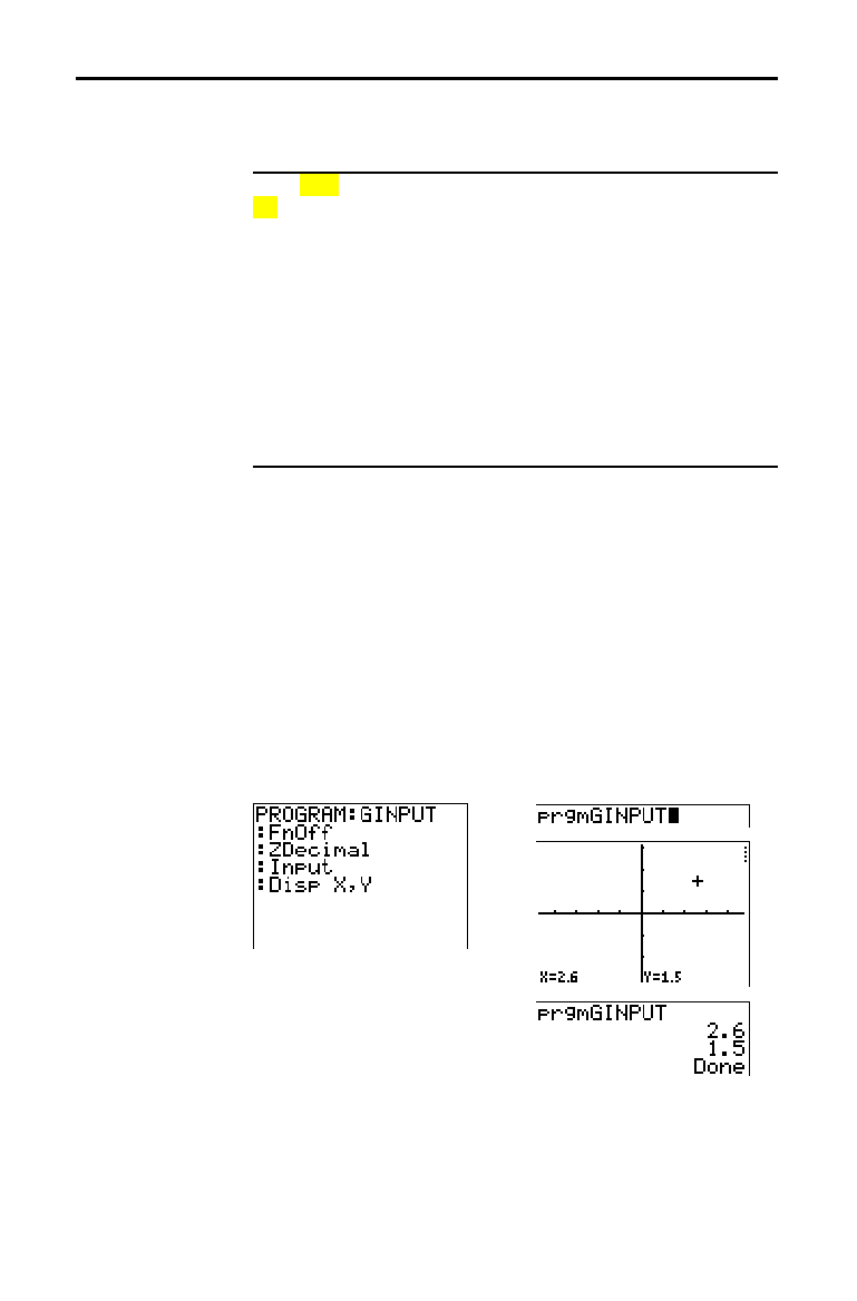
16-16 Programming
8316PROG.DOC TI-83 international English Bob Fedorisko Revised: 02/19/01 1:23 PM Printed: 02/19/01 1:39
PM Page 16 of 22
To display the
PRGM I/O
(program input/output) menu,
press
~
from within the program editor only.
CTL I/O EXEC
1: Input
Enters a value or uses the cursor.
2: Prompt
Prompts for entry of variable values.
3: Disp
Displays text, value, or the home screen.
4: DispGraph
Displays the current graph.
5: DispTable
Displays the current table.
6: Output(
Displays text at a specified position.
7: getKey
Checks the keyboard for a keystroke.
8: ClrHome
Clears the display.
9: ClrTable
Clears the current table.
0: GetCalc(
Gets a variable from another TI
-
83.
A: Get(
Gets a variable from CBL 2/CBL or CBR.
B: Send(
Sends a variable to CBL 2/CBL or CBR.
These instructions control input to and output from a
program during execution. They allow you to enter values
and display answers during program execution.
To return to the program editor without selecting an item,
press
‘
.
Input without a variable displays the current graph. You
can move the free-moving cursor, which updates
X and Y
(and R and
q
for PolarGC format). The pause indicator is
on. Press
Í
to resume program execution.
Input
Program Output
PRGM I/O (Input/Output) Instructions
PRGM I/O Menu
Displaying a
Graph with Input
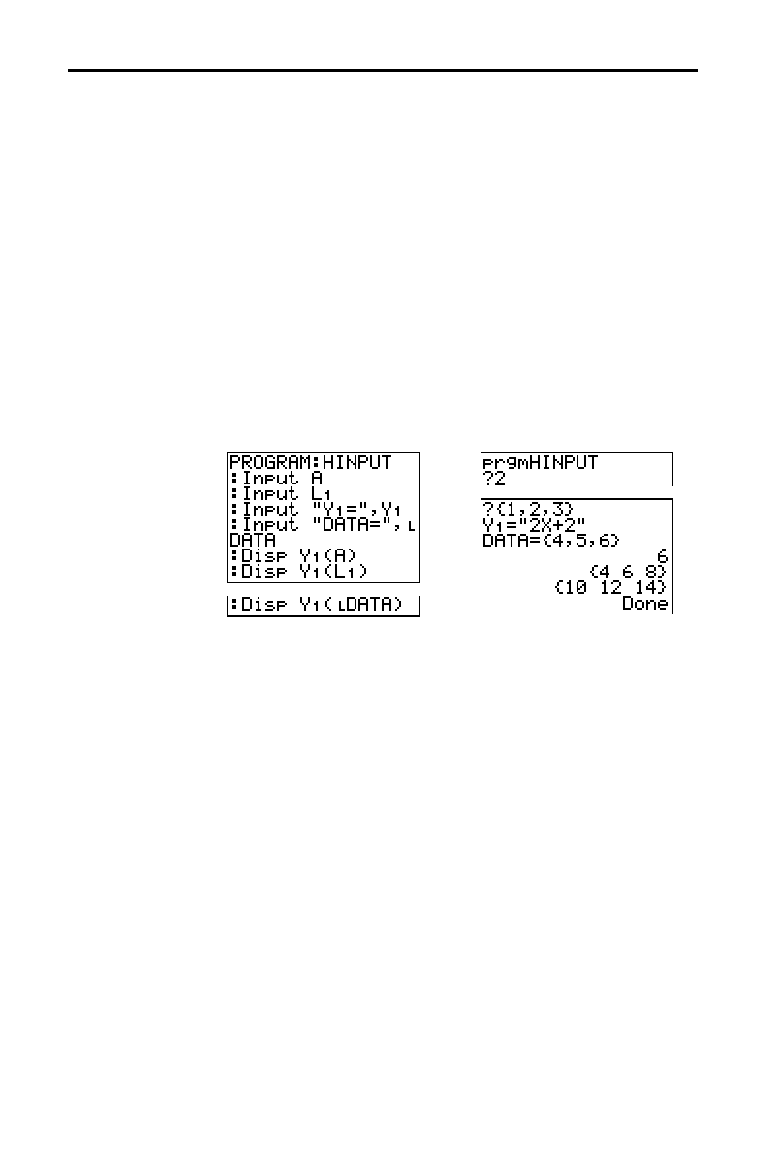
Programming 16-17
8316PROG.DOC TI-83 international English Bob Fedorisko Revised: 02/19/01 1:23 PM Printed: 02/19/01 1:39
PM Page 17 of 22
Input with
variable
displays a ? (question mark) prompt
during execution.
variable
may be a real number, complex
number, list, matrix, string, or
Y=
function. During program
execution, enter a value, which can be an expression, and
then press
Í
. The value is evaluated and stored to
variable
, and the program resumes execution.
Input [
variable
]
You can display
text
or the contents of
Str
n
(a string
variable) of up to 16 characters as a prompt. During
program execution, enter a value after the prompt and then
press
Í
. The value is stored to
variable
, and the
program resumes execution.
Input ["
text
",
variable
]
Input [Str
n
,
variable
]
Program Output
Note:
When a program prompts for input of lists and
Y
n
functions
during execution, you must include the braces (
{ }
) around the list
elements and quotation marks (
"
) around the expressions.
Storing a
Variable Value
with Input

16-18 Programming
8316PROG.DOC TI-83 international English Bob Fedorisko Revised: 02/19/01 1:23 PM Printed: 02/19/01 1:39
PM Page 18 of 22
During program execution, Prompt displays each
variable
,
one at a time, followed by
=?. At each prompt, enter a
value or expression for each
variable
, and then press
Í
. The values are stored, and the program resumes
execution.
Prompt
variableA
[,
variableB
,...,
variable n
]
Program Output
Note:
Y= functions are not valid with
Prompt
.
Disp (display) without a value displays the home screen.
To view the home screen during program execution, follow
the
Disp instruction with a Pause instruction.
Disp
Disp
with one or more
values
displays the value of each.
Disp [
valueA
,
valueB
,
valueC
,...,
value n
]
•
If
value
is a variable, the current value is displayed.
•
If
value
is an expression, it is evaluated and the result is
displayed on the right side of the next line.
•
If
value
is text within quotation marks, it is displayed on
the left side of the current display line.
!
is not valid as
text.
Program Output
If Pause is encountered after Disp, the program halts
temporarily so you can examine the screen. To resume
execution, press
Í
.
Note:
If a matrix or list is too large to display in its entirety, ellipses (
...
)
are displayed in the last column, but the matrix or list cannot be
scrolled. To scroll, use
Pause
value
(page 16
.
12).
Prompt
Displaying the
Home Screen
Displaying
Values and
Messages
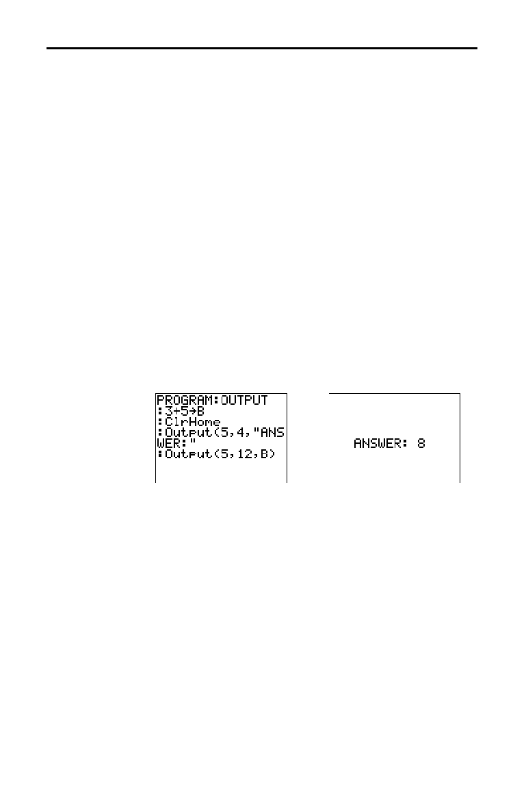
Programming 16-19
8316PROG.DOC TI-83 international English Bob Fedorisko Revised: 02/19/01 1:23 PM Printed: 02/19/01 1:39
PM Page 19 of 22
DispGraph (display graph) displays the current graph. If
Pause is encountered after DispGraph, the program halts
temporarily so you can examine the screen. Press
Í
to
resume execution.
DispTable (display table) displays the current table. The
program halts temporarily so you can examine the screen.
Press
Í
to resume execution.
Output( displays
text
or
value
on the current home screen
beginning at
row
(
1 through 8) and
column
(1 through 16),
overwriting any existing characters.
Tip:
You may want to precede
Output(
with
ClrHome
(page 16
.
20).
Expressions are evaluated and values are displayed
according to the current mode settings. Matrices are
displayed in entry format and wrap to the next line.
!
is
not valid as text.
Output(
row
,
column
,"
text
")
Output(
row
,
column
,
value
)
Program Output
For Output( on a Horiz split screen, the maximum value for
row
is 4.
DispGraph
DispTable
Output(
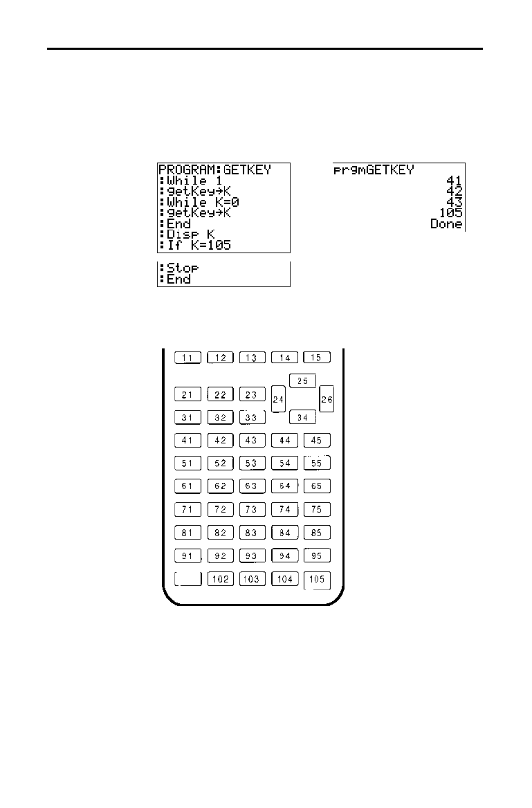
16-20 Programming
8316PROG.DOC TI-83 international English Bob Fedorisko Revised: 02/19/01 1:23 PM Printed: 02/19/01 1:39
PM Page 20 of 22
getKey returns a number corresponding to the last key
pressed, according to the key code diagram below. If no
key has been pressed,
getKey returns 0. Use getKey inside
loops to transfer control, for example, when creating video
games.
Program Output
Note:
,
,
, and
Í
were pressed during
program execution.
Note:
You can press
É
at any time during execution to break the
program (page 16
.
5).
ClrHome (clear home screen) clears the home screen
during program execution.
ClrTable (clear table) clears the values in the table during
program execution.
getKey
TI-83 Key Code
Diagram
ClrHome,
ClrTable
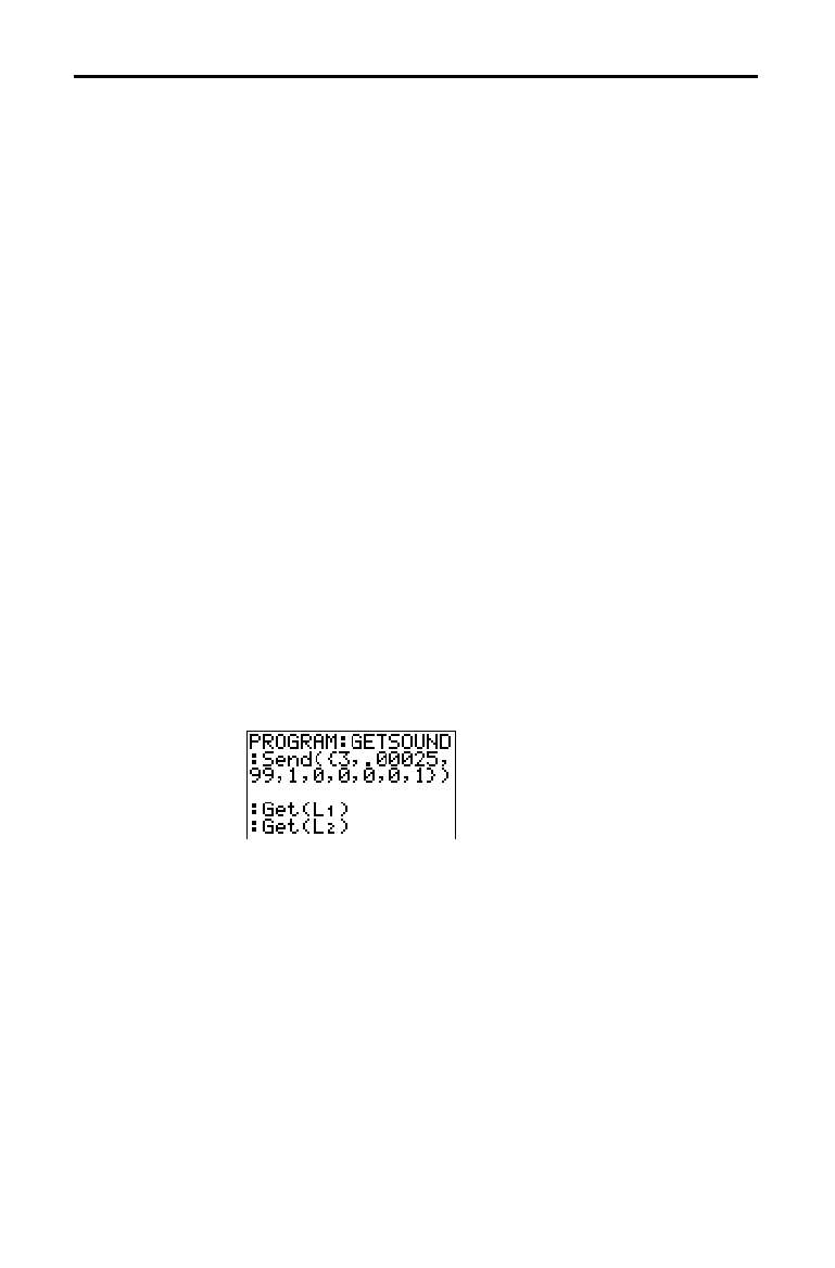
Programming 16-21
8316PROG.DOC TI-83 international English Bob Fedorisko Revised: 02/19/01 1:23 PM Printed: 02/19/01 1:39
PM Page 21 of 22
GetCalc( gets the contents of
variable
on another TI
-
83 and
stores it to
variable
on the receiving TI
-
83.
variable
can be
a real or complex number, list element, list name, matrix
element, matrix name, string,
Y=
variable, graph database,
or picture.
GetCalc(
variable
)
Note:
GetCalc(
does not work between TI
.
82s and TI
-
83s.
Get( gets data
from the Calculator-Based Laboratory
é
(CBL 2
é
, CBL
é
) System or Calculator-Based Ranger
é
(CBR
é
) and stores it to
variable
on the receiving TI
-
83.
variable
can be a real number, list element, list name,
matrix element, matrix name, string,
Y=
variable, graph
database, or picture.
Get(
variable
)
Note:
If you transfer a program that references the
Get(
command to
the TI
-
83 from a TI
.
82, the TI
-
83 will interpret it as the
Get(
described
above. Use
GetCalc(
to get data from another TI
-
83.
Send( sends the contents of
variable
to the CBL 2/CBL or
CBR. You cannot use it to send to another TI
-
83.
variable
can be a real number, list element, list name, matrix
element, matrix name, string,
Y=
variable, graph database,
or picture.
variable
can be a list of elements.
Send(
variable
)
Note:
This program gets sound data
and time in seconds from
CBL 2/CBL.
Note:
You can access
Get(
,
Send(
, and
GetCalc(
from the
CATALOG
to execute them from the home screen (Chapter 15).
GetCalc(
Get(, Send(
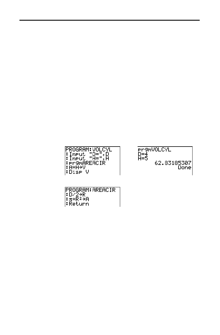
16-22 Programming
8316PROG.DOC TI-83 international English Bob Fedorisko Revised: 02/19/01 1:23 PM Printed: 02/19/01 1:39
PM Page 22 of 22
On the TI
-
83, any stored program can be called from
another program as a subroutine. Enter the name of the
program to use as a subroutine on a line by itself.
You can enter a program name on a command line in either
of two ways.
•
Press
|
to display the
PRGM EXEC
menu and
select the name of the program (page 16
.
7). prgm
name
is
pasted to the current cursor location on a command line.
•
Select
prgm from the
PRGM CTL
menu, and then enter
the program name (page 16
.
15).
prgm
name
When
prgm
name
is encountered during execution, the next
command that the program executes is the first command
in the second program. It returns to the subsequent
command in the first program when it encounters either
Return or the implied Return at the end of the second
program.
Program Output
&
Subroutine
(
'
Variables are global.
label
used with
Goto and Lbl is local to the program where
it is located.
label
in one program is not recognized by
another program. You cannot use
Goto to branch to a
label
in another program.
Return exits a subroutine and returns to the calling
program, even if it is encountered within nested loops.
Calling Other Programs as Subroutines
Calling a
Program from
Another Program
Notes about
Calling Programs
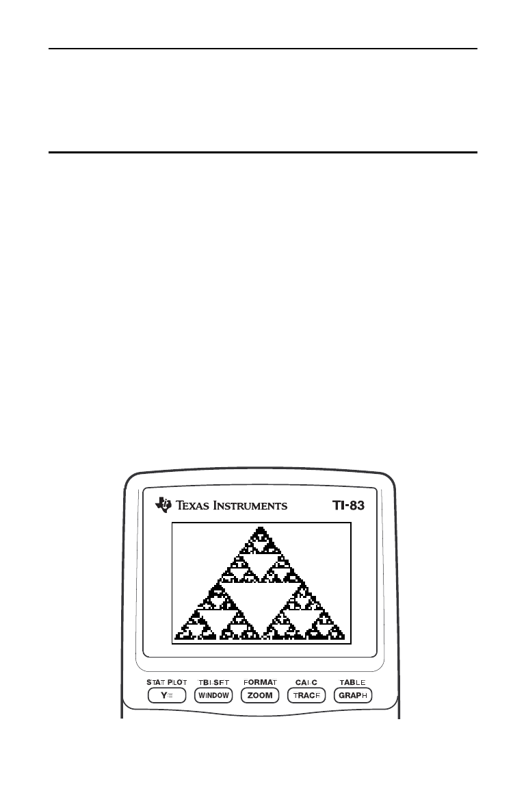
Applications 17-1
8317APPS.DOC TI-83 international English Bob Fedorisko Revised: 02/19/01 1:00 PM Printed: 02/19/01 1:39 PM
Page 1 of 20
17
Applications
Comparing Test Results Using Box Plots
................
17-2
Graphing Piecewise Functions
...........................
17-4
Graphing Inequalities
....................................
17-5
Solving a System of Nonlinear Equations
................
17-6
Using a Program to Create the Sierpinski Triangle
.......
17-7
Graphing Cobweb Attractors
............................
17-8
Using a Program to Guess the Coefficients
...............
17-9
Graphing the Unit Circle and Trigonometric Curves
......
17-10
Finding the Area between Curves
........................
17-11
Using Parametric Equations: Ferris Wheel Problem
......
17-12
Demonstrating the Fundamental Theorem of Calculus
...
17-14
Computing Areas of Regular N-Sided Polygons
..........
17-16
Computing and Graphing Mortgage Payments
...........
17-18
Contents
17-2 Applications
8317APPS.DOC TI-83 international English Bob Fedorisko Revised: 02/19/01 1:00 PM Printed: 02/19/01 1:39 PM
Page 2 of 20
An experiment found a significant difference between boys
and girls pertaining to their ability to identify objects held
in their left hands, which are controlled by the right side of
their brains, versus their right hands, which are controlled
by the left side of their brains. The TI Graphics team
conducted a similar test for adult men and women.
The test involved 30 small objects, which participants were
not allowed to see. First, they held 15 of the objects one by
one in their left hands and guessed what they were. Then
they held the other 15 objects one by one in their right hands
and guessed what they were. Use box plots to compare
visually the correct-guess data from this table.
Correct Guesses
Women
Left
Women
Right
Men
Left
Men
Right
84 712
91 86
12 8 7 12
11 12 5 12
10 11 7 7
811 811
12 13 11 12
712 48
9111012
11 12 14 11
13 9
59
1. Press
…
5
to select
5:SetUpEditor
. Enter list names
WLEFT
,
WRGHT
,
MLEFT
, and
MRGHT
, separated by
commas. Press
Í
. The stat list editor now contains
only these four lists.
2. Press
…
1
to select
1:Edit
.
3. Enter into
WLEFT
the number of correct guesses each
woman made using her left hand (
Women Left
). Press
~
to move to
WRGHT
and enter the number of correct
guesses each woman made using her right hand (
Women
Right
).
4. Likewise, enter each man’s correct guesses in
MLEFT
(
Men Left)
and
MRGHT
(
Men Right
).
5. Press
y
[
STAT PLOT
]. Select
1:Plot1
. Turn on plot 1;
define it as a modified box plot
Õ
that uses
WLEFT
.
Move the cursor to the top line and select
Plot2
. Turn on
plot 2; define it as a modified box plot that uses
WRGHT
.
Comparing Test Results Using Box Plots
Problem
Procedure
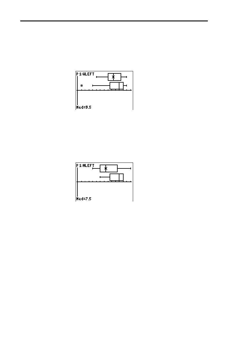
Applications 17-3
8317APPS.DOC TI-83 international English Bob Fedorisko Revised: 02/19/01 1:00 PM Printed: 02/19/01 1:39 PM
Page 3 of 20
6. Press
o
. Turn off all functions.
7. Press
p
. Set
Xscl=1 and Yscl=0. Press
q
9 to
select
9:ZoomStat. This adjusts the viewing window and
displays the box plots for the women’s results.
8. Press
r
.
%
Women’s left-hand data
%
Women’s right-hand data
Use
|
and
~
to examine minX, Q
1
, Med, Q
3
, and maxX
for each plot. Notice the outlier to the women’s right-
hand data. What is the median for the left hand? For the
right hand? With which hand were the women more
accurate guessers, according to the box plots?
9. Examine the men’s results. Redefine plot 1 to use
MLEFT, redefine plot 2 to use MRGHT. Press
r
.
%
Men’s left-hand data
%
Men’s right-hand data
Press
|
and
~
to examine minX, Q
1
, Med, Q
3
, and maxX
for each plot. What difference do you see between the
plots?
10.Compare the left-hand results. Redefine plot 1 to use
WLEFT, redefine plot 2 to use MLEFT, and then press
r
to examine
minX, Q
1
, Med, Q
3
, and maxX for each
plot. Who were the better left-hand guessers, men or
women?
11.Compare the right-hand results. Define plot 1 to use
WRGHT, define plot 2 to use MRGHT, and then press
r
to examine
minX, Q
1
, Med, Q
3
, and maxX for each
plot. Who were the better right-hand guessers?
In the original experiment boys did not guess as well
with right hands, while girls guessed equally well with
either hand. This is not what our box plots show for
adults. Do you think that this is because adults have
learned to adapt or because our sample was not large
enough?
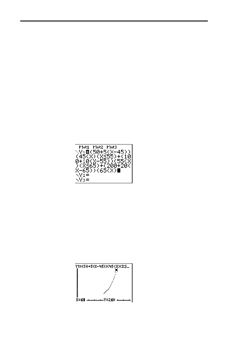
17-4 Applications
8317APPS.DOC TI-83 international English Bob Fedorisko Revised: 02/19/01 1:00 PM Printed: 02/19/01 1:39 PM
Page 4 of 20
The fine for speeding on a road with a speed limit of 45
kilometers per hour (kph) is 50; plus 5 for each kph from
46 to 55 kph; plus 10 for each kph from 56 to 65 kph; plus
20 for each kph from 66 kph and above. Graph the
piecewise function that describes the cost of the ticket.
The fine (Y) as a function of kilometers per hour (X) is:
Y = 0 0 < X
45
Y = 50 + 5 (X
N
45) 45 < X
55
Y = 50 + 5
…
10 + 10 (X
N
55) 55 < X
65
Y = 50 + 5
…
10 + 10
…
10 + 20 (X
N
65) 65 < X
1. Press
z
. Select
Func and the default settings.
2. Press
o
. Turn off all functions and stat plots. Enter the
Y=
function to describe the fine. Use the
TEST
menu
operations to define the piecewise function. Set the
graph style for
Y
1
to
í
(dot).
3. Press
p
and set Xmin=
L
2, Xscl=10, Ymin=
L
5, and
Yscl=10. Ignore Xmax and Ymax; they are set by
@
X
and
@
Y
in step 4.
4. Press
y
[
QUIT
] to return to the home screen. Store 1 to
@
X
, and then store 5 to
@
Y
.
@
X
and
@
Y
are on the
VARS Window X/Y
secondary menu.
@
X
and
@
Y
specify
the horizontal and vertical distance between the centers
of adjacent pixels. Integer values for
@
X
and
@
Y
produce
nice values for tracing.
5. Press
r
to plot the function. At what speed does
the ticket exceed 250?
Graphing Piecewise Functions
Problem
Procedure
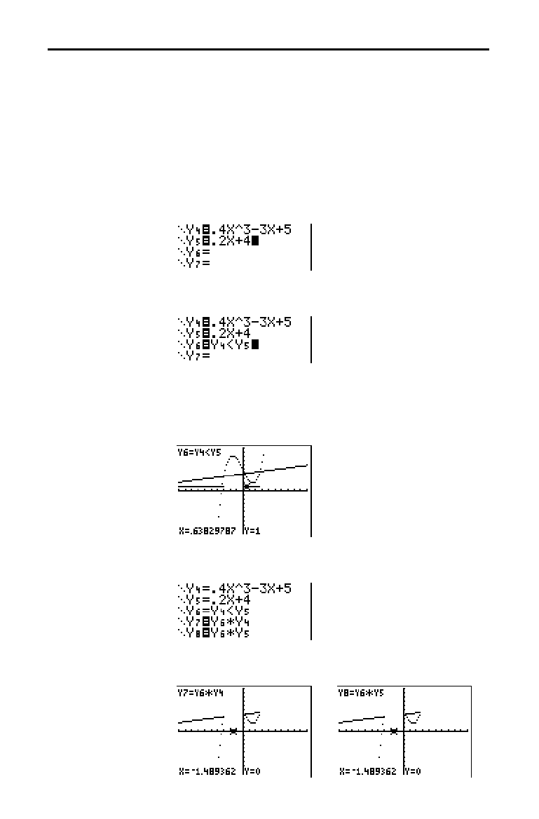
Applications 17-5
8317APPS.DOC TI-83 international English Bob Fedorisko Revised: 02/19/01 1:00 PM Printed: 02/19/01 1:39 PM
Page 5 of 20
Graph the inequality 0
.
4X
3
N
3X + 5 < 0
.
2X + 4. Use the
TEST
menu operations to explore the values of X where the
inequality is true and where it is false.
1. Press
z
. Select
Dot, Simul, and the default settings.
Setting
Dot mode changes all graph style icons to
í
(dot) in the
Y=
editor.
2. Press
o
. Turn off all functions and stat plots. Enter the
left side of the inequality as
Y
4
and the right side as Y
5
.
3. Enter the statement of the inequality as Y
6
. This
function evaluates to
1 if true or 0 if false.
4. Press
q
6 to graph the inequality in the standard
window.
5. Press
r
†
†
to move to
Y
6
. Then press
|
and
~
to trace the inequality, observing the value of
Y.
6. Press
o
. Turn off Y
4
, Y
5
, and Y
6
. Enter equations to
graph only the inequality.
7. Press
r
. Notice that the values of Y
7
and Y
8
are
zero where the inequality is false.
Graphing Inequalities
Problem
Procedure
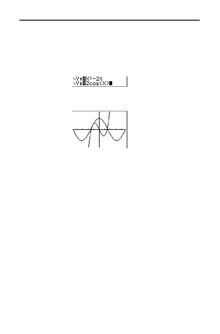
17-6 Applications
8317APPS.DOC TI-83 international English Bob Fedorisko Revised: 02/19/01 1:00 PM Printed: 02/19/01 1:39 PM
Page 6 of 20
Using a graph, solve the equation X
3
N
2X = 2cos(X). Stated
another way, solve the system of two equations and two
unknowns: Y = X
3
N
2X and Y = 2cos(X). Use
ZOOM
factors
to control the decimal places displayed on the graph.
1. Press
z
. Select the default mode settings. Press
o
.
Turn off all functions and stat plots. Enter the functions.
2. Press
q
4 to select 4:ZDecimal. The display shows
that two solutions may exist (points where the two
functions appear to intersect).
3. Press
q
~
4 to select 4:SetFactors from the
ZOOM
MEMORY
menu. Set XFact=10 and YFact=10.
4. Press
q
2 to select 2:Zoom In. Use
|
,
~
,
}
, and
†
to move the free-moving cursor onto the apparent
intersection of the functions on the right side of the
display. As you move the cursor, notice that the
X and Y
values have one decimal place.
5. Press
Í
to zoom in. Move the cursor over the
intersection. As you move the cursor, notice that now
the
X and Y values have two decimal places.
6. Press
Í
to zoom in again. Move the free-moving
cursor onto a point exactly on the intersection. Notice
the number of decimal places.
7. Press
y
[
CALC
] 5 to select 5:intersect. Press
Í
to
select the first curve and
Í
to select the second
curve. To guess, move the trace cursor near the
intersection. Press
Í
. What are the coordinates of
the intersection point?
8. Press
q
4 to select 4:ZDecimal to redisplay the
original graph.
9. Press
q
. Select
2:Zoom In and repeat steps 4
through 8 to explore the apparent function intersection
on the left side of the display.
Solving a System of Nonlinear Equations
Problem
Procedure
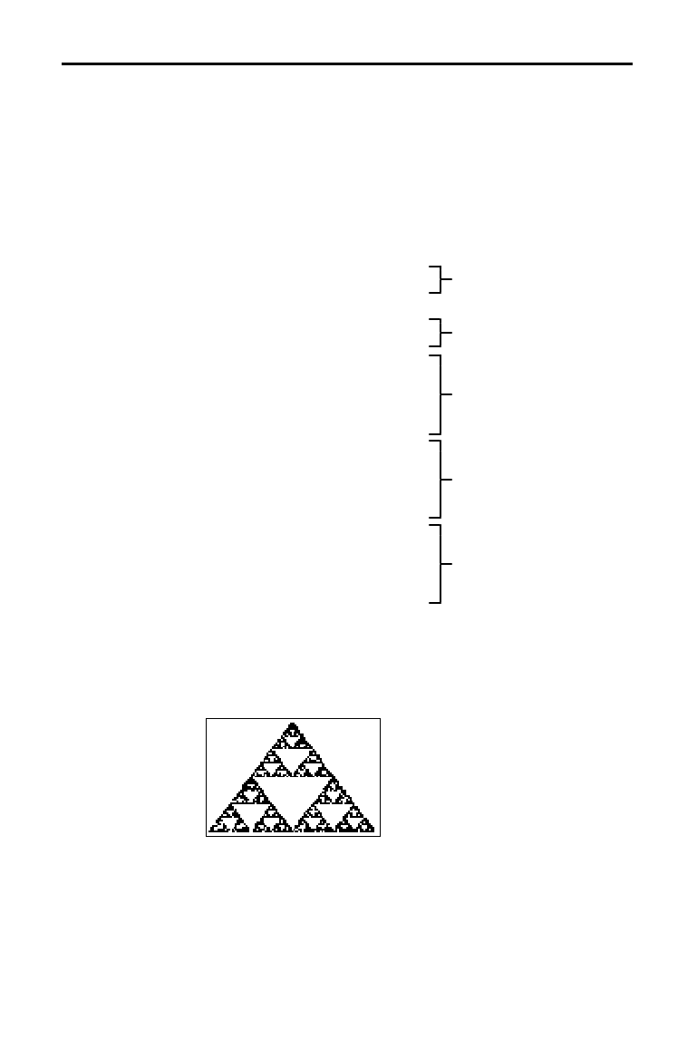
Applications 17-7
8317APPS.DOC TI-83 international English Bob Fedorisko Revised: 02/19/01 1:00 PM Printed: 02/19/01 1:39 PM
Page 7 of 20
This program creates a drawing of a famous fractal, the
Sierpinski Triangle, and stores the drawing to a picture. To
begin, press
~
~
1. Name the program SIERPINS,
and then press
Í
. The program editor is displayed.
PROGRAM:SIERPINS
:FnOff :ClrDraw
:PlotsOff
:AxesOff
:0
!
Xmin:1
!
Xmax
:0
!
Ymin:1
!
Ymax
Set viewing window.
:rand
!
X:rand
!
Y
:For(K,1,3000)
:rand
!
N
Beginning of For group.
:If N
1
à
3
:Then
:.5X
!
X
:.5Y
!
Y
:End
If/Then group
:If 1
à
3 <N and N
2
à
3
:Then
:.5(.5+X)
!
X
:.5(1+Y)
!
Y
:End
If/Then group.
:If 2
à
3<N
:Then
:.5(1+X)
!
X
:.5Y
!
Y
:End
If/Then group.
:Pt-On(X,Y)
Draw point.
:End
End of For group.
:StorePic 6
Store picture.
After you execute the program above, you can recall and
display the picture with the instruction
RecallPic 6.
Using a Program to Create the Sierpinski Triangle
Setting up the
Program
Program
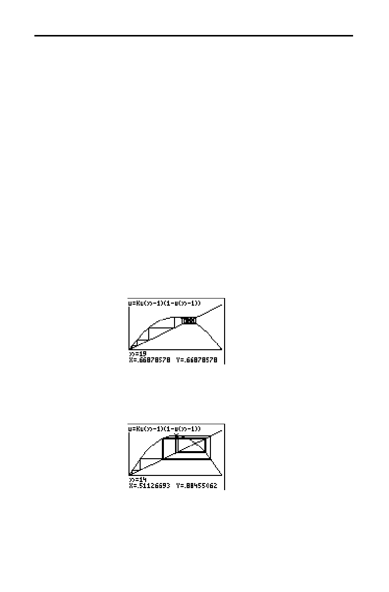
17-8 Applications
8317APPS.DOC TI-83 international English Bob Fedorisko Revised: 02/19/01 1:00 PM Printed: 02/19/01 1:39 PM
Page 8 of 20
Using Web format, you can identify points with attracting
and repelling behavior in sequence graphing.
1. Press
z
. Select
Seq and the default mode settings.
Press
y
[
FORMAT
]. Select Web format and the default
format settings.
2. Press
o
. Clear all functions and turn off all stat plots.
Enter the sequence that corresponds to the expression
Y = K X(1
N
X).
u(
n
)=Ku(
n
N
1)(1
N
u(
n
N
1))
u(
n
Min)=.01
3. Press
y
[
QUIT
] to return to the home screen, and then
store
2.9 to K.
4. Press
p
. Set the window variables.
n
Min=0 Xmin=0 Ymin=
M
.26
n
Max=10 Xmax=1 Ymax=1.1
PlotStart=1 Xscl=1 Yscl=1
PlotStep=1
5. Press
r
to display the graph, and then press
~
to
trace the cobweb. This is a cobweb with one attractor.
6. Change K to 3.44 and trace the graph to show a cobweb
with two attractors.
7. Change
K to 3.54 and trace the graph to show a cobweb
with four attractors.
Graphing Cobweb Attractors
Problem
Procedure
Applications 17-9
8317APPS.DOC TI-83 international English Bob Fedorisko Revised: 02/19/01 1:00 PM Printed: 02/19/01 1:39 PM
Page 9 of 20
This program graphs the function A sin(BX) with random
integer coefficients between 1 and 10. Try to guess the
coefficients and graph your guess as C sin(DX). The
program continues until your guess is correct.
PROGRAM:GUESS
:PlotsOff :Func
:FnOff :Radian
:ClrHome
:"Asin(BX)"
!
Y1
:"Csin(DX)"
!
Y2
Define equations.
:GraphStyle(1,1)
:GraphStyle(2,5)
Set line and path
g
raph
styles.
:FnOff 2
:randInt(1,10)
!
A
:randInt(1,10)
!
B
:0
!
C:0
!
D
Initialize coefficients.
:
L
2
p!
Xmin
:2
p!
Xmax
:
pà
2
!
Xscl
:
L
10
!
Ymin
:10
!
Ymax
:1
!
Yscl
Set viewing window.
:DispGraph
:Pause
Display graph.
:FnOn 2
:Lbl Z
:Prompt C,D
Prompt for guess.
:DispGraph
:Pause
Display graph.
:If C=A
:Text(1,1,"C IS OK")
:If C
ƒ
A
:Text(1,1,"C IS WRONG")
:If D=B
:Text(1,50,"D IS OK")
:If D
ƒ
B
:Text(1,50,"D IS WRONG")
Display results.
:DispGraph
:Pause
Display graph.
:If C=A and D=B
:Stop
:Goto Z
Quit if
g
uesses are
correct.
Using a Program to Guess the Coefficients
Setting Up the
Program
Program
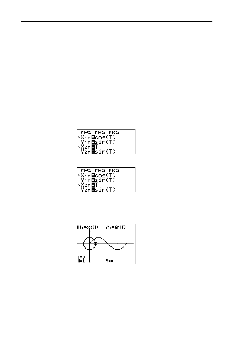
17-10 Applications
8317APPS.DOC TI-83 international English Bob Fedorisko Revised: 02/19/01 1:00 PM Printed: 02/19/01 1:39 PM
Page 10 of 20
Using parametric graphing mode, graph the unit circle and
the sine curve to show the relationship between them.
Any function that can be plotted in
Func mode can be
plotted in
Par mode by defining the X component as T and
the
Y component as F(T).
1. Press
z
. Select
Par, Simul, and the default settings.
2. Press
p
. Set the viewing window.
Tmin=0 Xmin=
L
2 Ymin=
L
3
Tmax=2
p
Xmax=7.4 Ymax=3
Tstep=.1 Xscl=
pà
2 Yscl=1
3. Press
o
. Turn off all functions and stat plots. Enter the
expressions to define the unit circle centered on (0,0).
4. Enter the expressions to define the sine curve.
5. Press
r
. As the graph is plotting, you may press
Í
to pause and
Í
again to resume graphing as
you watch the sine function “unwrap” from the unit
circle.
Note:
You can generalize the unwrapping. Replace
sin(T)
in
Y
2T
with
any other trig function to unwrap that function.
Graphing the Unit Circle and Trigonometric Curves
Problem
Procedure

Applications 17-11
8317APPS.DOC TI-83 international English Bob Fedorisko Revised: 02/19/01 1:00 PM Printed: 02/19/01 1:39 PM
Page 11 of 20
Find the area of the region bounded by
f(x) = 300x / (x
2
+ 625)
g(x) = 3cos(
.
1x)
x = 75
1. Press
z
. Select the default mode settings.
2. Press
p
. Set the viewing window.
Xmin=0 Ymin=
L
5
Xmax=100 Ymax=10
Xscl=10 Yscl=1
Xres=1
3. Press
o
. Turn off all functions and stat plots. Enter the
upper and lower functions.
Y
1
=300X
à
(X
2
+625)
Y
2
=3cos(.1X)
4. Press
y
[
CALC
] 5 to select 5:Intersect. The graph is
displayed. Select a first curve, second curve, and guess
for the intersection toward the left side of the display.
The solution is displayed, and the value of
X at the
intersection, which is the lower limit of the integral, is
stored in
Ans and X.
5. Press
y
[
QUIT
] to go to the home screen. Press
y
[
DRAW
] 7 and use Shade( to see the area graphically.
Shade(Y
2
,Y
1
,Ans,75)
6. Press
y
[
QUIT
] to return to the home screen. Enter the
expression to evaluate the integral for the shaded
region.
fnInt(Y
1
–Y
2
,X,Ans,75)
The area is 325.839962.
Finding the Area between Curves
Problem
Procedure
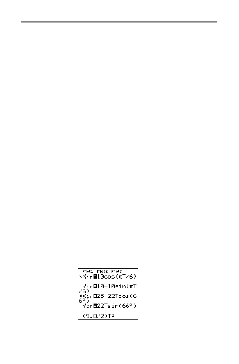
17-12 Applications
8317APPS.DOC TI-83 international English Bob Fedorisko Revised: 02/19/01 1:00 PM Printed: 02/19/01 1:39 PM
Page 12 of 20
Using two pairs of parametric equations, determine when
two objects in motion are closest to each other in the same
plane.
A ferris wheel has a diameter (d) of 20 meters and is
rotating counterclockwise at a rate (s) of one revolution
every 12 seconds. The parametric equations below
describe the location of a ferris wheel passenger at time T,
where
a
is the angle of rotation, (0,0) is the bottom center
of the ferris wheel, and (10,10) is the passenger’s location
at the rightmost point, when T=0.
X(T) = r cos
a
where
a
= 2
p
Ts and r = d
à
2
Y(T) = r + r sin
a
A person standing on the ground throws a ball to the ferris
wheel passenger. The thrower’s arm is at the same height as
the bottom of the ferris wheel, but 25 meters (b) to the right
of the ferris wheel’s lowest point (25,0). The person throws
the ball with velocity (v
0
) of 22 meters per second at an
angle (
q
) of 66
¡
from the horizontal. The parametric
equations below describe the location of the ball at time T.
X(T) = b
N
Tv
0
cos
q
Y(T) = Tv
0
sin
q
N
(g
à
2) T
2
where g =
9.8 m/ sec
2
1. Press
z
. Select Par, Simul, and the default settings.
Simul (simultaneous) mode simulates the two objects in
motion over time.
2. Press
p
. Set the viewing window.
Tmin=0 Xmin=
L
13 Ymin=0
Tmax=12 Xmax=34 Ymax=31
Tstep=.1 Xscl=10 Yscl=10
3. Press
o
. Turn off all functions and stat plots. Enter the
expressions to define the path of the ferris wheel and the
path of the ball. Set the graph style for
X
2T
to
ë
(path).
Tip:
Try setting the graph styles to
ë
X
1T
and
ì
X
2T
, which simulates a
chair on the ferris wheel and the ball flying through the air when you
press
s
.
Using Parametric Equations: Ferris Wheel Problem
Problem
Procedure
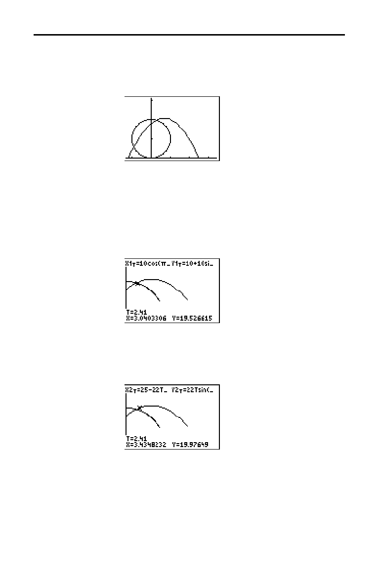
Applications 17-13
8317APPS.DOC TI-83 international English Bob Fedorisko Revised: 02/19/01 1:00 PM Printed: 02/19/01 1:39 PM
Page 13 of 20
4. Press
s
to graph the equations. Watch closely as
they are plotted. Notice that the ball and the ferris
wheel passenger appear to be closest where the paths
cross in the top-right quadrant of the ferris wheel.
5. Press
p
. Change the viewing window to
concentrate on this portion of the graph.
Tmin=1 Xmin=0 Ymin=10
Tmax=3 Xmax=23.5 Ymax=25.5
Tstep=.03 Xscl=10 Yscl=10
6. Press
r
. After the graph is plotted, press
~
to
move near the point on the ferris wheel where the paths
cross. Notice the values of
X, Y, and T.
7. Press
†
to move to the path of the ball. Notice the
values of
X and Y (T is unchanged). Notice where the
cursor is located. This is the position of the ball when
the ferris wheel passenger passes the intersection. Did
the ball or the passenger reach the intersection first?
You can use
r
to, in effect, take snapshots in time
and explore the relative behavior of two objects in
motion.
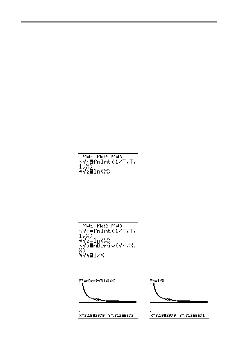
17-14 Applications
8317APPS.DOC TI-83 international English Bob Fedorisko Revised: 02/19/01 1:00 PM Printed: 02/19/01 1:39 PM
Page 14 of 20
Using the functions fnInt( and nDeriv( from the
MATH
menu
to graph functions defined by integrals and derivatives
demonstrates graphically that:
F(x) =
‰
1
x
1
à
t dt = ln(x), x > 0 and that
D
x
[
‰
1
x
1
à
t dt
]
= 1
à
x
1. Press
z
. Select the default settings.
2. Press
p
. Set the viewing window.
Xmin=.01 Ymin=
M
1.5 Xres=3
Xmax=10 Ymax=2.5
Xscl=1 Yscl=1
3. Press
o
. Turn off all functions and stat plots. Enter the
numerical integral of 1
à
T from 1 to X and the function
ln(X). Set the graph style for
Y
1
to
ç
(line) and Y
2
to
ë
(path).
4. Press
r
. Press
|
,
}
,
~
, and
†
to compare the
values of
Y
1
and Y
2
.
5. Press
o
. Turn off
Y
1
and Y
2
, and then enter the
numerical derivative of the integral of 1
à
X and the
function 1
à
X. Set the graph style for
Y
3
to
ç
(line) and Y
4
to
è
(thick).
6. Press
r
. Again, use the cursor keys to compare the
values of the two graphed functions,
Y
3
and Y
4
.
Demonstrating the Fundamental Theorem of Calculus
Problem 1
Procedure 1
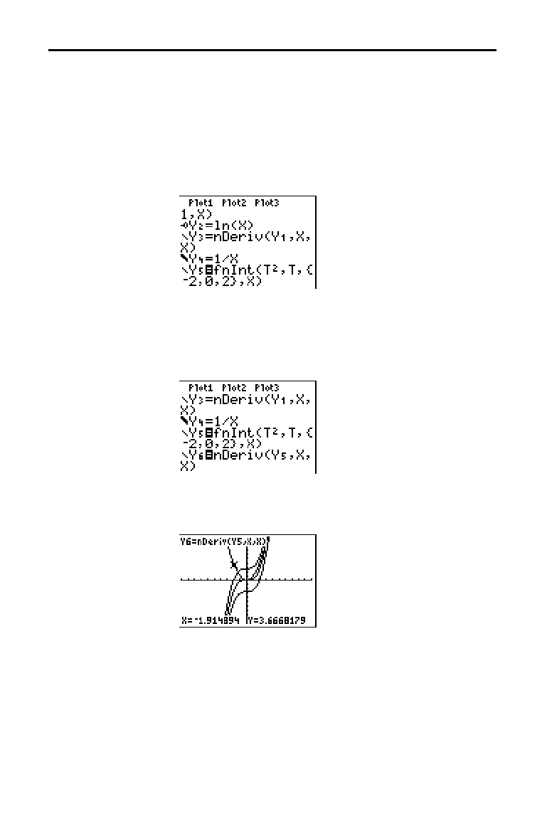
Applications 17-15
8317APPS.DOC TI-83 international English Bob Fedorisko Revised: 02/19/01 1:00 PM Printed: 02/19/01 1:39 PM
Page 15 of 20
Explore the functions defined by
y =
‰
M
2
x
t
2
dt,
‰
0
x
t
2
dt, and
‰
2
x
t
2
dt
1. Press
o
. Turn off all functions and stat plots. Use a list
to define these three functions simultaneously. Store
the function in
Y
5.
2. Press
q
6 to select 6:ZStandard.
3. Press
r
. Notice that the functions appear identical,
only shifted vertically by a constant.
4. Press
o
. Enter the numerical derivative of
Y
5
in Y
6
.
5. Press
r
. Notice that although the three graphs
defined by
Y
5
are different, they share the same
derivative.
Problem 2
Procedure 2
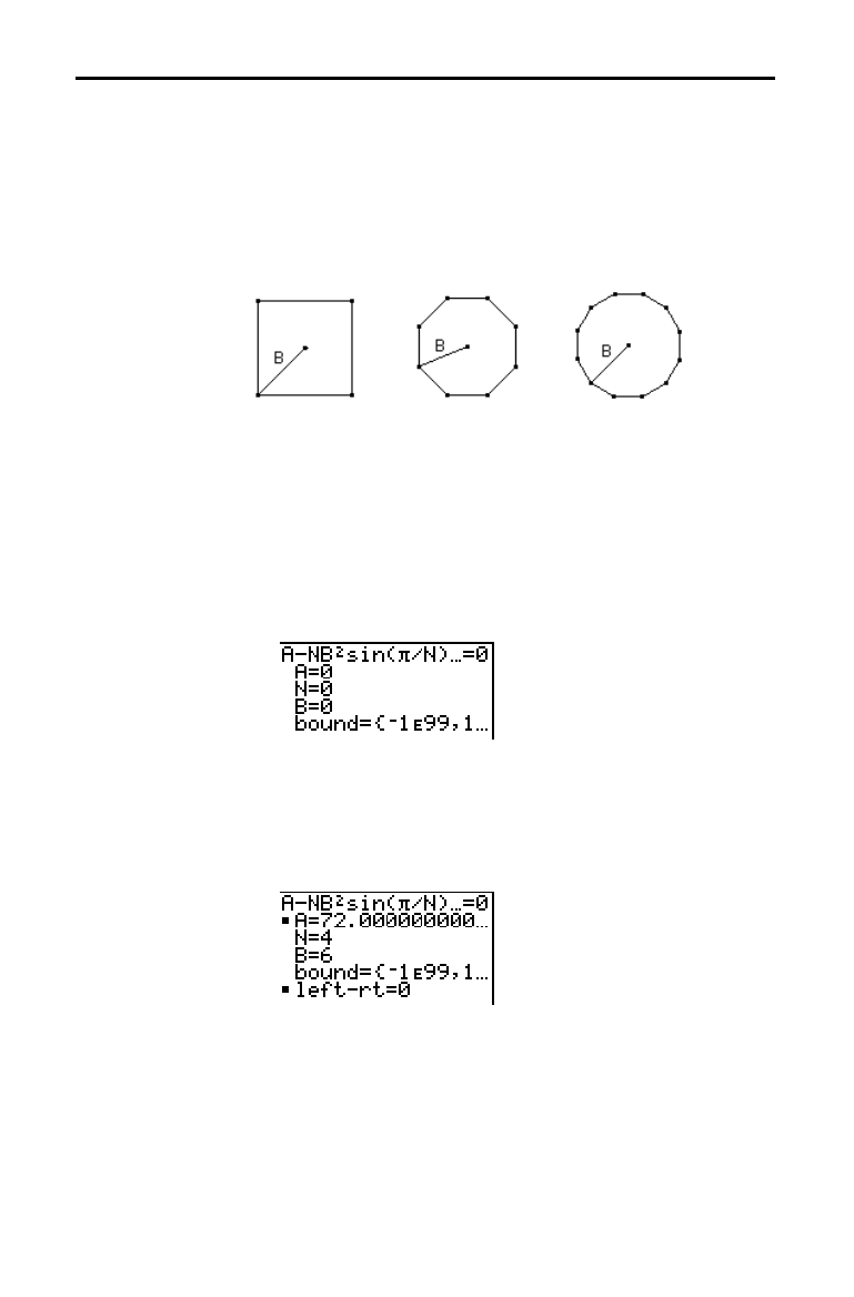
17-16 Applications
8317APPS.DOC TI-83 international English Bob Fedorisko Revised: 02/19/01 1:00 PM Printed: 02/19/01 1:39 PM
Page 16 of 20
Use the equation solver to store a formula for the area of a
regular N-sided polygon, and then solve for each variable,
given the other variables. Explore the fact that the limiting
case is the area of a circle,
p
r
2
.
Consider the formula A = NB
2
sin(
pà
N) cos(
pà
N) for the
area of a regular polygon with N sides of equal length and
B distance from the center to a vertex.
N = 4 sides N = 8 sides N = 12 sides
1. Press
0 to select 0:Solver from the
MATH
menu.
Either the equation editor or the interactive solver
editor is displayed. If the interactive solver editor is
displayed, press
}
to display the equation editor.
2. Enter the formula as
0=A
N
NB
2
sin(
p
/ N)cos(
p
/ N), and
then press
Í
. The interactive solver editor is
displayed.
3. Enter N=4 and B=6 to find the area (A) of a square with
a distance (
B) from center to vertex of 6 centimeters.
4. Press
}
}
to move the cursor onto
A, and then press
ƒ
[
SOLVE
]. The solution for A is displayed on the
interactive solver editor.
5. Now solve for B for a given area with various number of
sides. Enter
A=200 and N=6. To find the distance B,
move the cursor onto
B, and then press
ƒ
[
SOLVE
].
6. Enter
N=8. To find the distance B, move the cursor onto
B, and then press
ƒ
[
SOLVE
]. Find B for N=9, and
then for
N=10.
Computing Areas of Regular N-Sided Polygons
Problem
Procedure
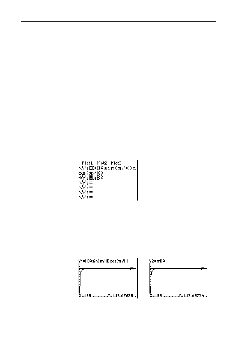
Applications 17-17
8317APPS.DOC TI-83 international English Bob Fedorisko Revised: 02/19/01 1:00 PM Printed: 02/19/01 1:39 PM
Page 17 of 20
Find the area given B=6, and N=10, 100, 150, 1000, and
10000. Compare your results with
p
6
2
(the area of a circle
with radius 6), which is approximately 113.097.
7. Enter
B=6. To find the area A, move the cursor onto A,
and then press
ƒ
[
SOLVE
]. Find A for N=10, then
N=100, then N=150, then N=1000, and finally N=10000.
Notice that as
N gets large, the area A approaches
p
B
2
.
Now graph the equation to see visually how the area
changes as the number of sides gets large.
8. Press
z
. Select the default mode settings.
9. Press
p
. Set the viewing window.
Xmin=0 Ymin=0 Xres=1
Xmax=200 Ymax=150
Xscl=10 Yscl=10
10.Press
o
. Turn off all functions and stat plots. Enter the
equation for the area. Use
X in place of N. Set the graph
styles as shown.
11.Press
r
. After the graph is plotted, press 100
Í
to trace to
X=100. Press 150
Í
. Press 188
Í
.
Notice that as
X increases, the value of Y converges to
p
6
2
, which is approximately 113.097. Y
2
=
p
B
2
(the area of
the circle) is a horizontal asymptote to
Y
1
. The area of
an N-sided regular polygon, with r as the distance from
the center to a vertex, approaches the area of a circle
with radius r (
p
r
2
) as N gets large.
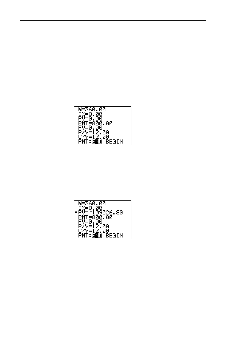
17-18 Applications
8317APPS.DOC TI-83 international English Bob Fedorisko Revised: 02/19/01 1:00 PM Printed: 02/19/01 1:39 PM
Page 18 of 20
You are a loan officer at a mortgage company, and you
recently closed on a 30-year home mortgage at 8 percent
interest with monthly payments of 800. The new home
owners want to know how much will be applied to the
interest and how much will be applied to the principal
when they make the 240th payment 20 years from now.
1. Press
z
and set the fixed-decimal mode to
2 decimal
places. Set the other mode settings to the defaults.
2. Press
y
[
FINANCE
] 1 to display the
TVM Solver
. Enter
these values.
Note:
Enter a positive number (
800
) to show
PMT
as a cash
inflow. Payment values will be displayed as positive numbers on
the graph. Enter
0
for
FV
, since the future value of a loan is 0 once
it is paid in full. Enter
PMT: END
, since payment is due at the end
of a period.
3. Move the cursor onto the PV= prompt, and then press
ƒ
[
SOLVE
]. The present value, or mortgage amount,
of the house is displayed at the
PV= prompt.
Computing and Graphing Mortgage Payments
Problem
Procedure
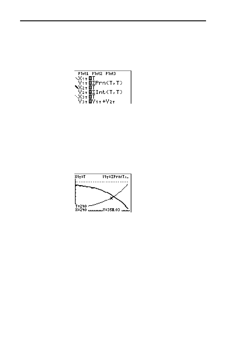
Applications 17-19
8317APPS.DOC TI-83 international English Bob Fedorisko Revised: 02/19/01 1:00 PM Printed: 02/19/01 1:39 PM
Page 19 of 20
Now compare the graph of the amount of interest with the
graph of the amount of principal for each payment.
4. Press
z
. Set
Par and Simul.
5. Press
o
. Turn off all functions and stat plots. Enter
these equations and set the graph styles as shown.
Note:
G
Prn(
and
G
Int(
are located on the
FINANCE CALC
menu.
6. Press
p
. Set these window variables.
Tmin=1 Xmin=0 Ymin=0
Tmax=360 Xmax=360 Ymax=1000
Tstep=12 Xscl=10 Yscl=100
Tip:
To increase the graph speed, change
Tstep
to
24
.
7. Press
r
. After the graph is drawn, press 240
Í
to move the trace cursor to
T=240, which is equivalent
to 20 years of payments.
The graph shows that for the 240th payment (X=240),
358.03 of the 800 payment is applied to principal
(
Y=358.03).
Note:
The sum of the payments (
Y
3T
=Y
1T
+Y
2T
) is always 800.
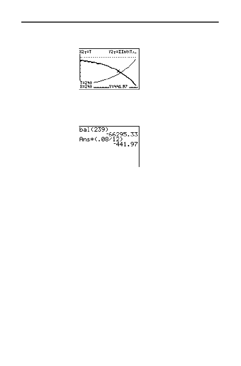
17-20 Applications
8317APPS.DOC TI-83 international English Bob Fedorisko Revised: 02/19/01 1:00 PM Printed: 02/19/01 1:39 PM
Page 20 of 20
8. Press
†
to move the cursor onto the function for
interest defined by
X
2T
and Y
2T
. Enter 240.
The graph shows that for the 240th payment (X=240),
441.97 of the 800 payment is interest (
Y=441.97).
9. Press
y
[
QUIT
]
y
[
FINANCE
] 9 to paste 9:bal( to the
home screen. Check the figures from the graph.
At which monthly payment will the principal allocation
surpass the interest allocation?
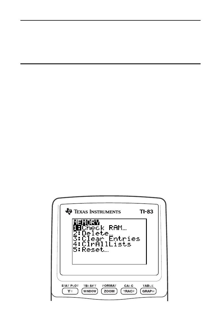
Memory Management 18-1
8318MEMR.DOC TI-83 international English Bob Fedorisko Revised: 02/19/01 1:01 PM Printed: 02/19/01 1:40
PM Page 1 of 6
18
Memor
y
Mana
g
ement
Checking Available Memory
.............................
18-2
Deleting Items from Memory
............................
18-3
Clearing Entries and List Elements
......................
18-4
Resetting the TI
-
83
......................................
18-5
Contents
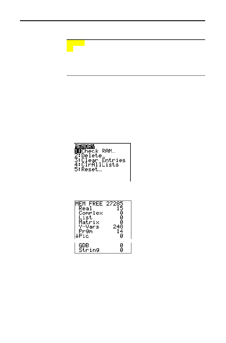
18-2 Memory Management
8318MEMR.DOC TI-83 international English Bob Fedorisko Revised: 02/19/01 1:01 PM Printed: 02/19/01 1:40
PM Page 2 of 6
To display the
MEMORY
menu, press
y
[
MEM
].
MEMORY
1: Check RAM
...
Reports memory availability/usage.
2: Delete
...
Displays
DELETE FROM
menu.
3: Clear Entries
Clears
ENTRY
(last-entry storage).
4: ClrAllLists
Clears all lists in memory.
5: Reset
...
Displays
RESET
menu (all/defaults).
Check RAM
displays the
Check RAM
screen. The top line
reports the total amount of available memory. The
remaining lines report the amount of memory each
variable type is using. You can check this screen to see
whether you need to delete variables from memory to
make room for new data, such as programs.
To check RAM usage, follow these steps.
1. Press
y
[
MEM
] to display the
MEMORY
menu.
2. Select
1:Check RAM
to display the
Check RAM
screen.
The TI
-
83 expresses memory quantities in bytes.
Note:
The
$
in the left column of
the bottom row indicates that you
can scroll or page down to view
more variable types.
Note:
Real
,
List
,
Y
.
Vars
, and
Prgm
variable types never reset to
zero, even after memory is cleared.
To leave the
Check RAM
screen, press either
y
[
QUIT
] or
‘
. Both options display the home screen.
Checking Available Memory
MEMORY Menu
Displaying the
Check RAM
Screen
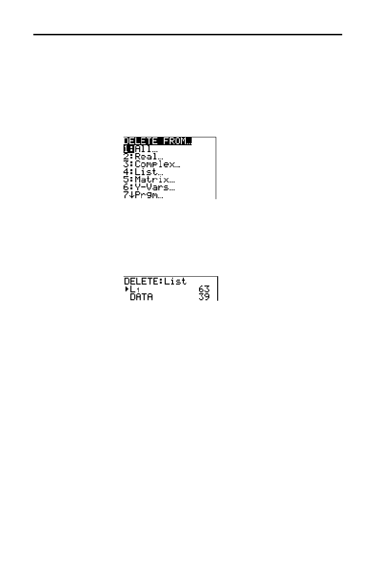
Memory Management 18-3
8318MEMR.DOC TI-83 international English Bob Fedorisko Revised: 02/19/01 1:01 PM Printed: 02/19/01 1:40
PM Page 3 of 6
To increase available memory by deleting the contents of
any variable (real or complex number, list, matrix,
Y=
variable, program, picture, graph database, or string),
follow these steps.
1. Press
y
[
MEM
] to display the
MEMORY
menu.
2. Select
2:Delete to display the
DELETE FROM
secondary
menu.
3. Select the type of data you want to delete, or select 1:All
for a list of all variables of all types. A screen is
displayed listing each variable of the type you selected
and the number of bytes each variable is using.
For example, if you select
4:List, the
DELETE:List
screen
is displayed.
4. Press
}
and
†
to move the selection cursor (
4
) next to
the item you want to delete, and then press
Í
. The
variable is deleted from memory. You can delete
individual variables one by one from this screen.
To leave any
DELETE:
screen without deleting anything,
press
y
[
QUIT
], which displays the home screen.
Note:
You cannot delete some system variables, such as the last-
answer variable
Ans
and the statistical variable
RegEQ
.
Deleting Items from Memory
Deleting an Item
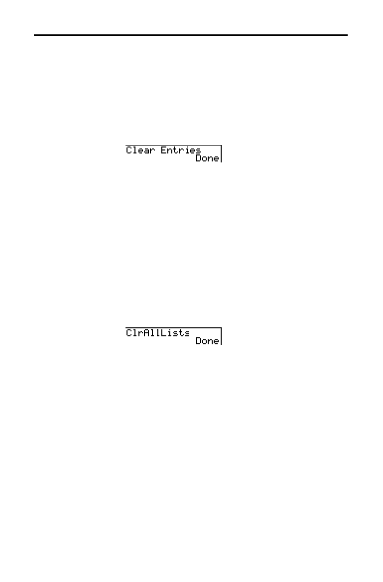
18-4 Memory Management
8318MEMR.DOC TI-83 international English Bob Fedorisko Revised: 02/19/01 1:01 PM Printed: 02/19/01 1:40
PM Page 4 of 6
Clear Entries clears the contents of the
ENTRY
(last entry)
storage area (Chapter 1). To clear the
ENTRY
storage area,
follow these steps.
1. Press
y
[
MEM
] to display the
MEMORY
menu.
2. Select
3:Clear Entries to paste the instruction to the
home screen.
3. Press
Í
to clear the
ENTRY
storage area.
To cancel Clear Entries, press
‘
.
Note:
If you select
3:Clear Entries
from within a program, the
Clear
Entries
instruction is pasted to the program editor, and the
Entry
(last entry) is cleared when the program is executed.
ClrAllLists sets to 0 the dimension of each list in memory.
To clear all elements from all lists, follow these steps.
1. Press
y
[
MEM
] to display the
MEMORY
menu.
2. Select
4:ClrAllLists to paste the instruction to the home
screen.
3. Press
Í
to set to
0 the dimension of each list in
memory.
To cancel ClrAllLists, press
‘
.
ClrAllLists does not delete list names from memory, from
the
LIST NAMES
menu, or from the stat list editor.
Note:
If you select
4:ClrAllLists
from within a program, the
ClrAllLists
instruction is pasted to the program editor. The lists are
cleared when the program is executed.
Clearing Entries and List Elements
Clear Entries
ClrAllLists
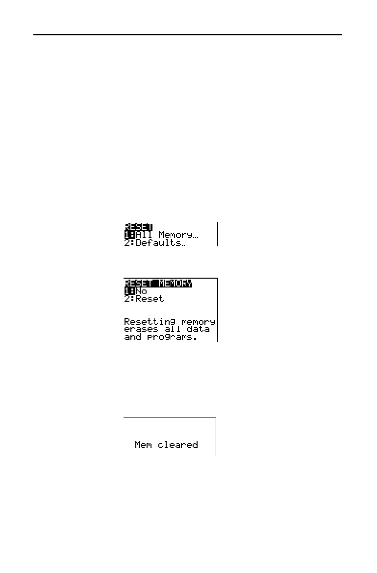
Memory Management 18-5
8318MEMR.DOC TI-83 international English Bob Fedorisko Revised: 02/19/01 1:01 PM Printed: 02/19/01 1:40
PM Page 5 of 6
The
RESET
secondary menu gives you the option of
resetting all memory (including default settings) or
resetting the default settings while preserving other data
stored in memory, such as programs and
Y=
functions.
Resetting all memory on the TI
-
83 restores memory to the
factory settings. It deletes all nonsystem variables and all
programs. It resets all system variables to the default
settings.
Tip:
Before you reset all memory, consider restoring sufficient
available memory by deleting only selected data (page 18
.
3).
To reset all memory on the TI
-
83, follow these steps.
1. Press
y
[
MEM
] to display the
MEMORY
menu.
2. Select
5:Reset
to display the
RESET
secondary menu.
3. Select
1:All Memory
to display the
RESET MEMORY
tertiary menu.
4. Read the message below the
RESET MEMORY
menu.
•
To cancel memory reset and return to the home
screen, select
1:No
.
•
To erase from memory all data and programs, select
2:Reset
. All factory defaults are restored.
Mem cleared
is displayed on the home screen.
Note:
When you clear memory, the contrast sometimes changes. If
the screen is faded or blank, adjust the contrast (Chapter 1).
Resetting the TI-83
RESET
Secondary Menu
Resetting All
Memory
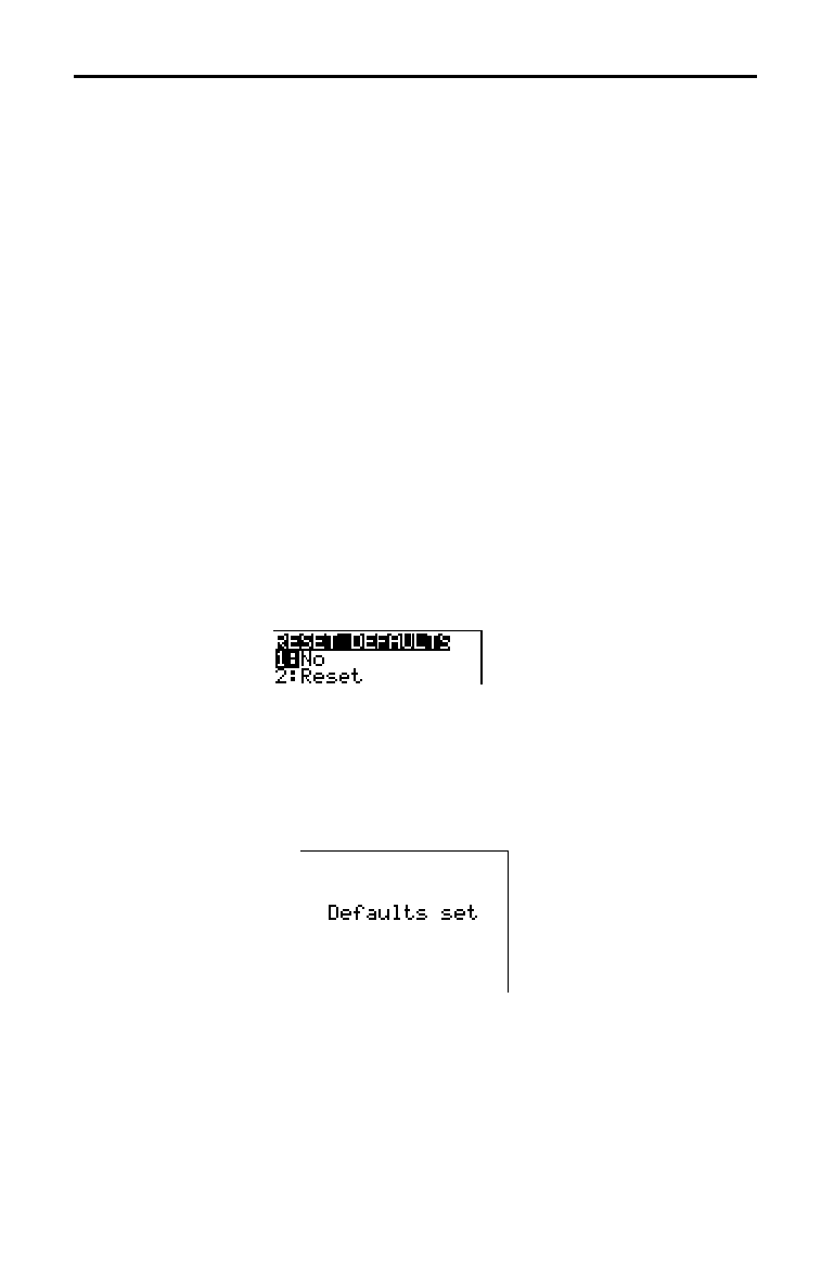
18-6 Memory Management
8318MEMR.DOC TI-83 international English Bob Fedorisko Revised: 02/19/01 1:01 PM Printed: 02/19/01 1:40
PM Page 6 of 6
When you reset defaults on the TI
-
83, all defaults are
restored to the factory settings. Stored data and programs
are not changed.
These are some examples of TI
-
83 defaults that are
restored by resetting the defaults.
•
Mode settings such as
Normal (notation); Func
(graphing); Real (numbers); and Full (screen)
•
Y=
functions off
•
Window variable values such as
Xmin=
L
10; Xmax=10;
Xscl=1; Yscl=1; and Xres=1
•
Stat plots off
•
Format settings such as
CoordOn (graphing coordinates
on); AxesOn; and ExprOn (expression on)
•
rand seed value to 0
To reset all TI
-
83 factory defaults, follow these steps.
1. Press
y
[
MEM
] to display the
MEMORY
menu.
2. Select
5:Reset to display the
RESET
secondary menu.
3. Select
2:Defaults to display the
RESET DEFAULTS
tertiary menu.
4. Consider the consequences of resetting defaults.
•
To cancel reset and return to the home screen, select
1:No.
•
To restore factory default settings, select
2:Reset.
Default settings are restored. Defaults set is
displayed on the home screen.
Resetting
Defaults
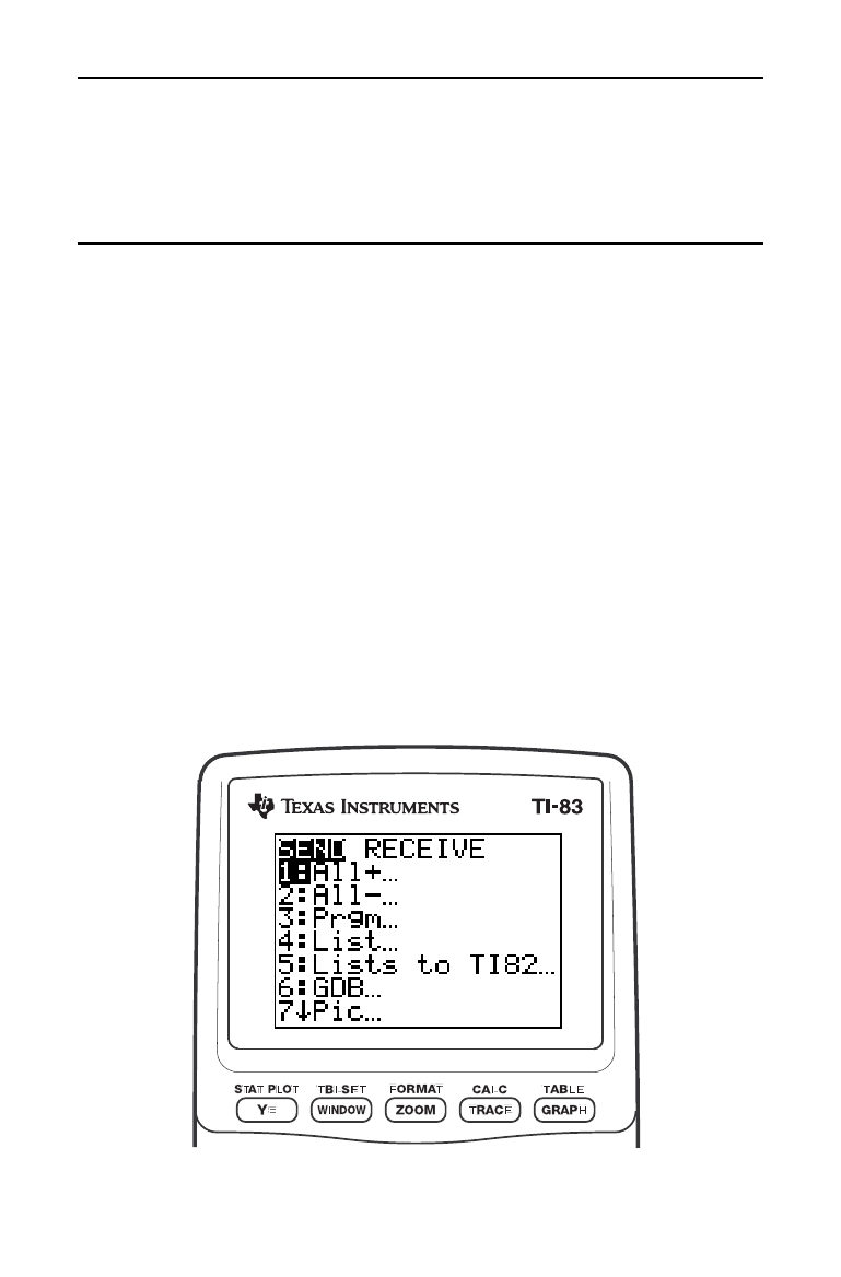
Communication Link 19-1
8319LINK.DOC TI-83 Intl English, Chap 19 Bob Fedorisko Revised: 02/19/01 1:24 PM Printed: 02/19/01 1:40 PM
Page 1 of 10
19
Communication
Link
Getting Started: Sending Variables
.......................
19-2
TI
-
83
LINK
...............................................
19-3
Selecting Items to Send
..................................
19-4
Receiving Items
..........................................
19-5
Transmitting Items
.......................................
19-6
Transmitting Lists to a TI
-
82
.............................
19-8
Transmitting from a TI
-
82 to a TI
-
83
.....................
19-9
Backing Up Memory
.....................................
19-10
Contents
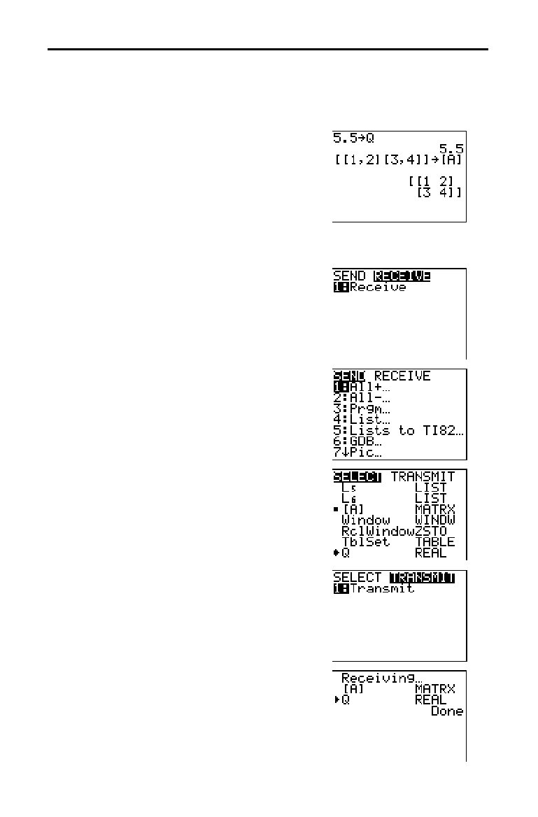
19-2 Communication Link
8319LINK.DOC TI-83 Intl English, Chap 19 Bob Fedorisko Revised: 02/19/01 1:24 PM Printed: 02/19/01 1:40 PM
Page 2 of 10
Getting Started is a fast-paced introduction. Read the chapter for details.
Create and store a variable and a matrix, and then transfer them to another
TI
-
83.
1. On the home screen of the sending unit,
press
5
Ë
5
¿
ƒ
Q. Press
Í
to
store 5.5 to
Q.
2. Press
y
[
[
]
y
[
[
] 1
¢
2
y
[
]
]
y
[
[
] 3
¢
4
y
[
]
]
y
[
]
]
¿
1.
Press
Í
to store the matrix to
[A].
3. Connect the calculators with the link
cable. Push both ends in firmly.
4. On the receiving unit, press
y
[
LINK
]
~
to
display the
RECEIVE
menu. Press 1 to
select
1:Receive. The message Waiting
...
is
displayed and the busy indicator is on.
5. On the sending unit, press
y
[
LINK
] to
display the
SEND
menu.
6. Press
2 to select 2:All
N
. The
All
N
SELECT
screen is displayed.
7. Press
†
until the selection cursor (
4
) is
next to
[A] MATRX. Press
Í
.
8. Press
†
until the selection cursor is next
to
Q REAL. Press
Í
. A square dot next
to
[A] and Q indicates that each is selected
to send.
9. On the sending unit, press
~
to display the
TRANSMIT
menu.
10. On the sending unit, press 1 to select
1:Transmit and begin transmission. The
receiving unit displays the message
Receiving....When the items are
transmitted, both units display the name
and type of each transmitted variable.
Getting Started: Sending Variables

Communication Link 19-3
8319LINK.DOC TI-83 Intl English, Chap 19 Bob Fedorisko Revised: 02/19/01 1:24 PM Printed: 02/19/01 1:40 PM
Page 3 of 10
The TI
-
83 has a port to connect and communicate with
another TI
-
83, a TI
-
82, the Calculator-Based Laboratory
é
(CBL 2
é
, CBL
é
) System, the Calculator-Based Ranger
é
(CBR
é
), or a personal computer. The unit-to-unit link
cable is included with the TI
-
83. This chapter describes
how to communicate with another calculator.
You can transfer all variables and programs to another
TI
-
83 or backup the entire memory of a TI
-
83. The
software that enables this communication is built into the
TI
-
83. To transmit from one TI
-
83 to another, follow the
steps on pages 19
.
6 and 19
.
7.
You can transfer from a TI
-
82 to a TI
-
83 all variables and
programs. Also, you can transfer from a TI
-
83 to a TI
-
82 lists
L
1
through L
6
.
The software that enables this communication is built into the
TI
-
83. To transmit data from a TI
-
82 to a TI
-
83, follow the
steps on pages 19
.
6 and 19
.
7.
•
You cannot perform a memory backup from a TI
-
82 to a
TI
-
83.
•
The only data type you can transmit from a TI
-
83 to a
TI
-
82 is list data stored in L
1
through L
6
. Use the
LINK
SEND
menu item 5:Lists to TI82 (page 19
.
8).
1. Insert either end of the cable into the port very firmly.
2. Insert the other end of the cable into the other
calculator’s port.
CBR and the CBL 2/CBL System are optional accessories
that connect to a TI
-
83 with the unit-to-unit link cable.
With a CBR or a CBL 2/CBL and a TI
-
83, you can collect
and analyze real-world data.
TI
.
GRAPH LINK
é
is an optional accessory that links a TI
-
83
to enable communication with a personal computer.
TI-83 LINK
TI-83 Link
Capabilities
Linking Two
TI-83s
Linking a TI-82
and a TI-83
Connecting Two
Calculators with
the Cable
Linking to a CBR
or the CBL 2/CBL
System
Linking to a PC
or Macintosh
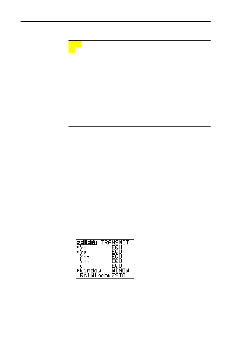
19-4 Communication Link
8319LINK.DOC TI-83 Intl English, Chap 19 Bob Fedorisko Revised: 02/19/01 1:24 PM Printed: 02/19/01 1:40 PM
Page 4 of 10
To display the
LINK SEND
menu, press
y
[
LINK
].
SEND RECEIVE
1: All+
...
Displays all items selected.
2: All
N
...
Displays all items deselected.
3: Prgm
...
Displays all programs names.
4: List
...
Displays all list names.
5: Lists to TI82
...
Displays list names
L
1
through
L
6
.
6: GDB
...
Displays all graph databases.
7: Pic
...
Displays all picture data types.
8: Matrix
...
Displays all matrix data types.
9: Real
...
Displays all real variables.
0: Complex
...
Displays all complex variables.
A: Y-Vars
...
Displays all
Y=
variables.
B: String
...
Displays all string variables.
C: Back Up
...
Selects all for backup to TI
-
83.
When you select an item on the
LINK SEND
menu, the
corresponding
SELECT
screen is displayed.
Note:
Each
SELECT
screen, except
All+ SELECT
, is displayed
initially with no data selected.
To select items to send on the sending unit, follow these
steps.
1. Press
y
[
LINK
] to display the
LINK SEND
menu.
2. Select the menu item that describes the data type to
send. The corresponding
SELECT
screen is displayed.
3. Press
}
and
†
to move the selection cursor (
4
) to an
item you want to select or deselect.
4. Press
Í
to select or deselect the item. Selected
names are marked with a
0
.
5. Repeat steps 3 and 4 to select or deselect additional items.
Selecting Items to Send
LINK SEND Menu
Selecting Items
to Send

Communication Link 19-5
8319LINK.DOC TI-83 Intl English, Chap 19 Bob Fedorisko Revised: 02/19/01 1:24 PM Printed: 02/19/01 1:40 PM
Page 5 of 10
To display the
LINK RECEIVE
menu, press
y
[
LINK
]
~
.
SEND RECEIVE
1: Receive
Sets unit to receive data transmission.
When you select
1:Receive from the
LINK RECEIVE
menu on
the receiving unit, the message
Waiting... and the busy
indicator are displayed. The receiving unit is ready to
receive transmitted items. To exit the receive mode
without receiving items, press
É
, and then select
1:Quit
from the
Error in Xmit
menu.
To transmit, follow the steps on page 19
.
6.
When transmission is complete, the unit exits the receive
mode. You can select
1:Receive again to receive more
items. The receiving unit then displays a list of items
received. Press
y
[
QUIT
] to exit the receive mode.
During transmission, if a variable name is duplicated, the
DuplicateName
menu is displayed on the receiving unit.
DuplicateName
1: Rename
Prompts to rename receiving variable.
2: Overwrite
Overwrites data in receiving variable.
3: Omit
Skips transmission of sending variable.
4: Quit
Stops transmission at duplicate variable.
When you select
1:Rename, the Name= prompt is displayed,
and alpha-lock is on. Enter a new variable name, and then
press
Í
. Transmission resumes.
When you select
2:Overwrite, the sending unit’s data
overwrites the existing data stored on the receiving unit.
Transmission resumes.
When you select
3:Omit, the sending unit does not send the
data in the duplicated variable name. Transmission
resumes with the next item.
When you select
4:Quit, transmission stops, and the
receiving unit exits receive mode.
During transmission, if the receiving unit does not have
sufficient memory to receive an item, the
Memory Full
menu
is displayed on the receiving unit.
•
To skip this item for the current transmission, select
1:Omit. Transmission resumes with the next item.
•
To cancel the transmission and exit receive mode,
select
2:Quit.
Receiving Items
LINK RECEIVE
Menu
Receiving Unit
DuplicateName
Menu
Insufficient
Memory in
Receiving Unit
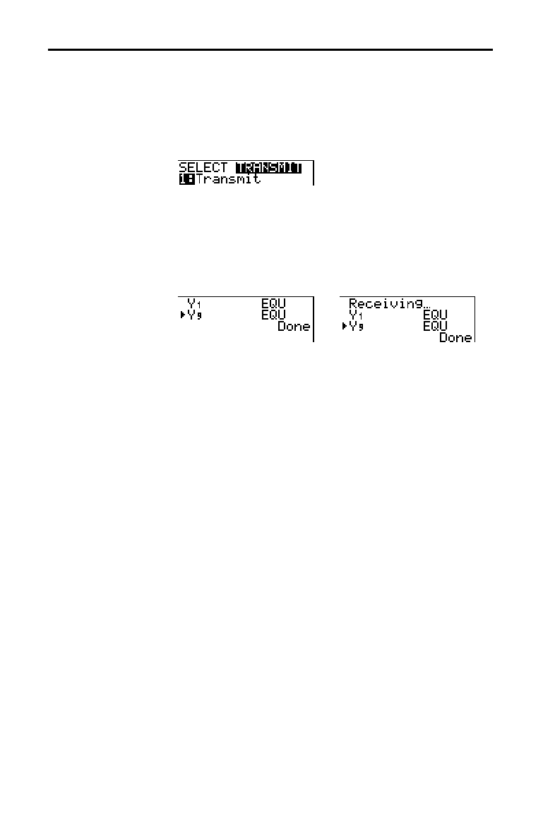
19-6 Communication Link
8319LINK.DOC TI-83 Intl English, Chap 19 Bob Fedorisko Revised: 02/19/01 1:24 PM Printed: 02/19/01 1:40 PM
Page 6 of 10
To transmit selected items after you have selected items to
send on the sending unit (page 19
.
4) and set the receiving
unit to receive (page 19
.
5), follow these steps.
1. Press
~
on the sending unit to display the
TRANSMIT
menu.
2. Confirm that Waiting... is displayed on the receiving
unit, which indicates it is set to receive (page 19
.
5).
3. Press
Í
to select
1:Transmit. The name and type of
each item are displayed line by line on the sending unit
as the item is queued for transmission, and then on the
receiving unit as each item is accepted.
After all selected items have been transmitted, the message
Done is displayed on both calculators. Press
}
and
†
to
scroll through the names.
To stop a link transmission, press
É
. The
Error in Xmit
menu is displayed on both units. To leave the error menu,
select
1:Quit.
A transmission error occurs after one or two seconds if:
•
A cable is not attached to the sending unit.
•
A cable is not attached to the receiving unit.
Note:
If the cable is attached, push it in firmly and try again.
•
The receiving unit is not set to receive transmission.
•
You attempt a backup between a TI
-
82 and a TI
-
83.
•
You attempt a data transfer from a TI
-
83 to a TI
-
82 with
data other than lists L
1
through L
6
or without using
menu item 5:Lists to TI82.
Although a transmission error does not occur, these two
conditions may prevent successful transmission.
•
You try to use
Get( with a calculator instead of a
CBL 2/CBL or CBR.
•
You try to use
GetCalc( with a TI
-
82 instead of a TI
-
83.
Transmitting Items
Transmitting
Items
Stopping a
Transmission
Error Conditions

Communication Link 19-7
8319LINK.DOC TI-83 Intl English, Chap 19 Bob Fedorisko Revised: 02/19/01 1:24 PM Printed: 02/19/01 1:40 PM
Page 7 of 10
After sending or receiving data, you can repeat the same
transmission to additional TI
-
83 units—from either the
sending unit or the receiving unit—without having to
reselect data to send. The current items remain selected.
Note:
You cannot repeat transmission if you selected All+ or All
.
.
To transmit to an additional TI
-
83, follow these steps.
1. Set the TI
-
83 to receive (page 19
.
5).
2. Do not select or deselect any new items to send. If you
select or deselect an item, all selections or deselections
from the previous transmission are cleared.
3. Disconnect the link cable from one TI
-
83 and connect it
to the additional TI
-
83.
4. Set the additional TI
-
83 to receive (page 19
.
5).
5. Press
y
[
LINK
] on the sending TI
-
83 to display the
LINK SEND
menu.
6. Select the menu item that you used for the last
transmission. The data from your last transmission is
still selected.
7. Press
~
to display the
LINK TRANSMIT
menu.
8. Confirm that the receiving unit is set to receive
(page 19
.
5).
9. Press
Í
to select
1:Transmit
and begin transmitting.
Transmitting
Items to an
Additional TI-83

19-8 Communication Link
8319LINK.DOC TI-83 Intl English, Chap 19 Bob Fedorisko Revised: 02/19/01 1:24 PM Printed: 02/19/01 1:40 PM
Page 8 of 10
The only data type you can transmit from a TI
-
83 to a TI
-
82
is list data stored in
L
1
through L
6
.
To transmit to a TI
-
82 the list data that is stored to TI
-
83
lists
L
1
, L
2
, L
3
, L
4
, L
5
, or L
6
, follow these steps.
1. Set the TI
-
82 to receive (page 19
.
5).
2. Press
y
[
LINK
] 5 on the sending TI
-
83 to select
5:Lists to TI82. The
SELECT
screen is displayed.
3. Select each list to transmit.
4. Press
~
to display the
LINK TRANSMIT
menu.
5. Confirm that the receiving unit is set to receive
(page 19
.
5).
6. Press
Í
to select
1:Transmit and begin transmitting.
Note:
If dimension > 99 for a TI
-
83 list that is selected to send, the
receiving TI
-
82 will truncate the list at the ninety-ninth element during
transmission.
Transmitting Lists to a TI-82
Transmitting
Lists to a TI-82

Communication Link 19-9
8319LINK.DOC TI-83 Intl English, Chap 19 Bob Fedorisko Revised: 02/19/01 1:24 PM Printed: 02/19/01 1:40 PM
Page 9 of 10
Generally, you can transmit items to a TI
-
83 from a TI
-
82,
but differences between the two products may affect some
transmitted data. This table shows differences for which
the software built into the TI
-
83 automatically adjusts
when a TI
-
83 receives TI
-
82 data.
TI
.
82 TI
.
83
n
Min PlotStart
n
Start
n
Min
U
n
u
V
n
v
U
n
Start u(
n
Min)
V
n
Start v(
n
Min)
TblMin TblStart
For example, if you transmit from a TI
-
82 to a TI
-
83 a
program that contains
n
Start
on a command line and then
display the program on the receiving TI
-
83, you will see
that
n
Min
has automatically replaced
n
Start
on the
command line.
The software built into the TI
-
83 cannot resolve some
differences between the TI
-
82 and TI
-
83, which are
described below. You must edit the data on the TI
-
83 after
you transmit to account for these differences, or the TI
-
83
will misinterpret the data.
The TI
-
83 reinterprets TI
-
82 prefix functions to include
open parentheses, which may add extraneous parentheses
to transmitted expressions.
For example, if you transmit
sin X+5
from a TI
-
82 to a
TI
.
83, the TI
-
83 reinterprets it as
sin(X+5
. Without a closing
parenthesis after
X
, the TI
-
83 interprets this as
sin(X+5)
, not
the sum of
5
and
sin(X)
.
If a TI
-
82 instruction that the TI
-
83 cannot translate is
transmitted, the
ERR:INVALID
menu is displayed when the
TI
-
83 attempts to execute the instruction. For example, on
the TI
-
82, the character group
U
n-1
is pasted to the cursor
location when you press
y
[
Un
N
1
]. The TI
-
83 cannot
directly translate
U
n-1
to the TI
-
83 syntax
u(n
N
1)
, so the
ERR:INVALID
menu is displayed.
Note:
TI
-
83 implied multiplication rules differ from those of the TI
.
82.
For example, the TI
-
83 evaluates
1
à
2X
as
(1
à
2)
ä
X
, while the TI
-
82
evaluates
1
à
2X
as
1
à
(2
ä
X)
(Chapter 2).
Transmitting from a TI-82 to a TI-83
Resolved
Differences
between the TI-82
and TI-83
Unresolved
Differences
between the TI-82
and TI-83
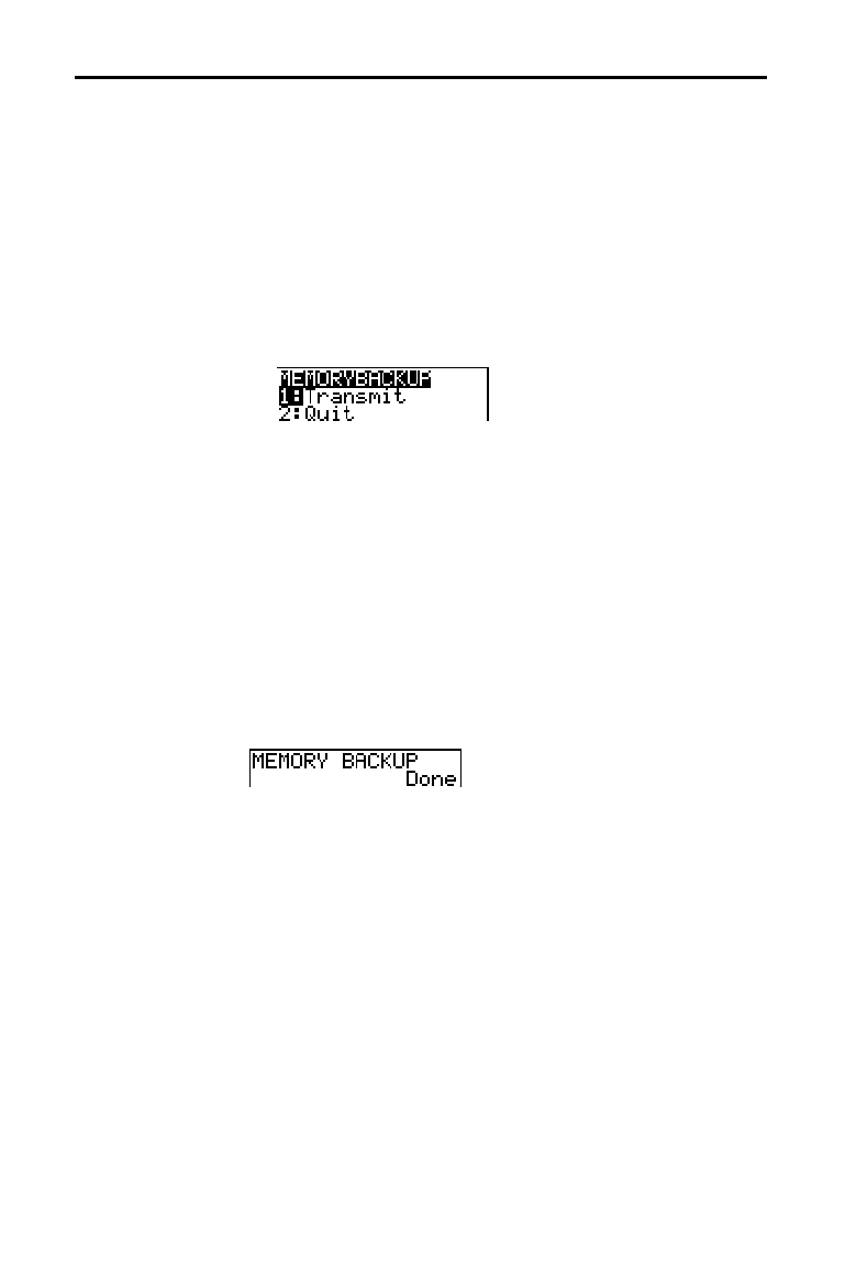
19-10 Communication Link
8319LINK.DOC TI-83 Intl English, Chap 19 Bob Fedorisko Revised: 02/19/01 1:24 PM Printed: 02/19/01 1:40 PM
Page 10 of 10
To copy the exact contents of memory in the sending TI
-
83
to the memory of the receiving TI
-
83, put the other unit in
receive mode. Then, on the receiving unit, select
C:Back Up
from the
LINK SEND
menu.
•
Warning:
C:Back Up overwrites the memory in the
receiving unit; all information in the memory of the
receiving unit is lost.
Note:
If you do not want to do a backup, select
2:Quit
to return to
the
LINK SEND
menu.
•
Select
1:Transmit to begin transmission.
As a safety check to prevent accidental loss of memory,
the message
WARNING
.
Backup is displayed when the
receiving unit receives notice of a backup.
•
To continue with the backup process, select
1:Continue.
The backup transmission begins.
•
To prevent the backup, select
2:Quit.
Note:
If a transmission error is returned during a backup, the receiving
unit is reset.
When the backup is complete, both the sending calculator
and receiving calculator display a confirmation screen.
Backing Up Memory
Memory Backup
Receiving Unit
Memory Backup
Complete

Tables and Reference Information A-1
8399APXA.DOC TI-83 international English Bob Fedorisko Revised: 02/19/01 1:25 PM Printed: 02/19/01 1:40 PM
Page 1 of 58
A
Tables and Reference
Information
Table of Functions and Instructions
.....................
A-2
TI
.
83 Menu Map
.........................................
A-39
Variables
................................................
A-49
Statistics Formulas
......................................
A-50
Financial Formulas
......................................
A-54
Contents

A-2 Tables and Reference Information
8399APXA.DOC TI-83 international English Bob Fedorisko Revised: 02/19/01 1:25 PM Printed: 02/19/01 1:40 PM
Page 2 of 58
Functions return a value, list, or matrix. You can use functions in an expression.
Instructions initiate an action. Some functions and instructions have arguments.
Optional arguments and accompanying commas are enclosed in brackets ( [ ] ).
For details about an item, including argument descriptions and restrictions, turn
to the page listed on the right side of the table.
From the
CATALOG
, you can paste any function or instruction to the home
screen or to a command line in the program editor. However, some functions
and instructions are not valid on the home screen. The items in this table
appear in the same order as they appear in the
CATALOG
.
† indicates keystrokes that are valid in the program editor only. Some keystrokes
display menus that are available only in the program editor. Others paste mode,
format, or table-set instructions only when you are in the program editor.
Function or Instruction/
Arguments Result
Key or Keys/
Menu or Screen/Item
abs(
value
)
Returns the absolute value of a
real number, expression, list,
or matrix.
NUM
1:abs(
2
-
13
10
-
10
abs(
complex value
)
Returns the magnitude of a
complex number or list.
CPX
5:abs(
2
-
19
valueA
and
valueB
Returns 1 if both
valueA
and
valueB
are
ƒ
0
.
valueA
and
valueB
can be real numbers,
expressions, or lists.
y
[
TEST
]
LOGIC
1:and
2
-
26
angle(
value
)
Returns the polar angle of a
complex number or list of
complex numbers.
CPX
4:angle(
2
-
19
ANOVA(
list1
,
list2
[
,
list3
,
...
,
list20
]
)
Performs a one-way analysis of
v
ariance for comparing the
means of two to 20
populations.
…
TESTS
F:ANOVA(
13
-
25
Ans
Returns the last answer.
y
[
ANS
] 1
-
18
Table of Functions and Instructions

Tables and Reference Information A-3
8399APXA.DOC TI-83 international English Bob Fedorisko Revised: 02/19/01 1:25 PM Printed: 02/19/01 1:40 PM
Page 3 of 58
Function or Instruction/
Arguments Result
Key or Keys/
Menu or Screen/Item
augment(
matrixA
,
matrixB
)
Returns a matrix, which is
matrixB
appended to
matrixA
as new columns.
MATH
7:augment(
10
-
14
augment(
listA
,
listB
)
Returns a list, which is
listB
concatenated to the end of
listA
.
y
[
LIST
]
OPS
9:augment(
11
-
15
AxesOff
Turns off the graph axes.
†
y
[
FORMAT
]
AxesOff
3
-
14
AxesOn
Turns on the graph axes.
†
y
[
FORMAT
]
AxesOn
3
-
14
a+b
i
Sets the mode to rectangular
complex number mode (a+b
i
).
†
z
a+b
i
1
-
12
bal(
npmt
[
,
roundvalue
]
)
Computes the balance at
npmt
for an amortization schedule
using stored values for
PV
,
æ
,
and
PMT
and rounds the
computation to
roundvalue.
y
[
FINANCE
]
CALC
9:bal(
14
-
9
binomcdf(
numtrials
,
p
[
,
x
]
)
Computes a cumulative
probability at
x
for the discrete
binomial distribution with the
specified
numtrials
and
probability
p
of success on
each trial.
y
[
DISTR
]
DISTR
A:binomcdf(
13
-
33
binompdf(
numtrials
,
p
[
,
x
]
)
Computes a probability at
x
for
the discrete binomial
distribution with the specified
numtrials
and probability
p
of
success on each trial.
y
[
DISTR
]
DISTR
0:binompdf(
13
-
33
c
2
cdf(
lowerbound
,
upperbound
,
df
)
Computes the
c
2
distribution
probability between
lowerbound
and
upperbound
for the specified degrees of
freedom
df
.
y
[
DISTR
]
DISTR
7:
c
2
cdf(
13
-
31

A-4 Tables and Reference Information
8399APXA.DOC TI-83 international English Bob Fedorisko Revised: 02/19/01 1:25 PM Printed: 02/19/01 1:40 PM
Page 4 of 58
Function or Instruction/
Arguments Result
Key or Keys/
Menu or Screen/Item
c
2
pdf(
x
,
df
)
Computes the probability
density function (pdf) for the
c
2
distribution at a specified
x
v
alue for the specified degrees
of freedom
df
.
y
[
DISTR
]
DISTR
6:
c
2
pdf(
13
-
31
c
2
.
Test(
observedmatrix
,
expectedmatrix
[
,
drawflag
]
)
Performs a chi-square test.
drawflag
=
1
draws results;
drawflag
=
0
calculates results.
†
…
TESTS
C:
c
2
.
Test(
13
-
22
Circle(
X
,
Y
,
radius
)
Draws a circle with center
(
X
,
Y
) and
radius
.
y
[
DRAW
]
DRAW
9:Circle(
8
-
11
Clear Entries
Clears the contents of the Last
Entry storage area.
y
[
MEM
]
MEMORY
3:Clear Entries
18
-
4
ClrAllLists
Sets to
0
the dimension of all
lists in memory.
y
[
MEM
]
MEMORY
4:ClrAllLists
18
-
4
ClrDraw
Clears all drawn elements from
a graph or drawing.
y
[
DRAW
]
DRAW
1:ClrDraw
8
-
4
ClrHome
Clears the home screen.
†
I/O
8:ClrHome
16
-
20
ClrList
listname1
[
,
listname2
, ...,
listname n
]
Sets to
0
the dimension of one
or more
listnames
.
…
EDIT
4:ClrList
12
-
20
ClrTable
Clears all values from the
table.
†
I/O
9:ClrTable
16
-
20
conj(
value
)
Returns the complex conjugate
of a complex number or list of
complex numbers.
CPX
1:conj(
2
-
18
Connected
Sets connected plotting mode;
resets all
Y=
editor graph-style
settings to
ç
.
†
z
Connected
1
-
11

Tables and Reference Information A-5
8399APXA.DOC TI-83 international English Bob Fedorisko Revised: 02/19/01 1:25 PM Printed: 02/19/01 1:40 PM
Page 5 of 58
Function or Instruction/
Arguments Result
Key or Keys/
Menu or Screen/Item
CoordOff
Turns off cursor coordinate
v
alue display.
†
y
[
FORMAT
]
CoordOff
3
-
14
CoordOn
Turns on cursor coordinate
v
alue display.
†
y
[
FORMAT
]
CoordOn
3
-
14
cos(
value
)
Returns cosine of a
real number, expression, or
list.
™
2
-
3
cos
L
1
(
value
)
Returns arccosine of a real
number, expression, or list.
y
[
COS
L
1
]
2
-
3
cosh(
value
)
Returns hyperbolic cosine of a
real number, expression, or
list.
y
[
CATALOG
]
cosh(
15
-
10
cosh
L
1
(
value
)
Returns hyperbolic arccosine
of a real number, expression,
or list.
y
[
CATALOG
]
cosh
L
1
(
15
-
10
CubicReg
[
Xlistname
,
Ylistname
,
freqlist
,
regequ
]
Fits a cubic regression model
to
Xlistname
and
Ylistname
with frequency
freqlist
, and
stores the regression equation
to
regequ
.
…
CALC
6:CubicReg
12
-
26
cumSum(
list
)
Returns a list of the cumulative
sums of the elements in
list
,
starting with the first element.
y
[
LIST
]
OPS
6:cumSum(
11-12
cumSum(
matrix
)
Returns a matrix of the
cumulative sums of
matrix
elements. Each element in the
returned matrix is a cumulative
sum of a
matrix
column from
top to bottom.
MATH
0:cumSum(
10
-
15
dbd(
date1
,
date2
)
Calculates the number of days
between
date1
and
date2
using
the actual-day-count method.
y
[
FINANCE
]
CALC
D:dbd(
14
-
13
value
4
Dec
Displays a real or complex
number, expression, list, or
matrix in decimal format.
MATH
2:
4
Dec
2
-
5

A-6 Tables and Reference Information
8399APXA.DOC TI-83 international English Bob Fedorisko Revised: 02/19/01 1:25 PM Printed: 02/19/01 1:40 PM
Page 6 of 58
Function or Instruction/
Arguments Result
Key or Keys/
Menu or Screen/Item
Degree
Sets degree angle mode.
†
z
Degree
1
-
11
DelVar
variable
Deletes from memory the
contents of
variable
.
†
CTL
G:DelVar
16
-
15
DependAsk
Sets table to ask for
dependent-variable values.
†
y
[
TBLSET
]
Depend: Ask
7
-
3
DependAuto
Sets table to generate
dependent-variable values
automatically.
†
y
[
TBLSET
]
Depend: Auto
7
-
3
det(
matrix
)
Returns determinant of
matrix
.
MATH
1:det(
10
-
12
DiagnosticOff
Sets diagnostics-off mode;
r
,
r
2
,
and
R
2
are not displayed as
regression model results.
y
[
CATALOG
]
DiagnosticOff
12
-
23
DiagnosticOn
Sets diagnostics-on mode;
r
,
r
2
,
and
R
2
are displayed as
regression model results.
y
[
CATALOG
]
DiagnosticOn
12
-
23
dim(
listname
)
Returns the dimension of
listname
.
y
[
LIST
]
OPS
3:dim(
11
-
11
dim(
matrixname
)
Returns the dimension of
matrixname
as a list.
MATH
3:dim(
10
-
12
length
!
dim(
listname
)
Assigns a new dimension
(
length
) to a new or existing
listname
.
y
[
LIST
]
OPS
3:dim(
11
-
11
{
rows
,
columns
}
!
dim(
matrixname
)
Assigns new dimensions to a
new or existing
matrixname
.
MATH
3:dim(
10
-
13
Disp
Displays the home screen.
†
I/O
3:Disp
16
-
18
Disp
[
valueA
,
valueB
,
valueC
,
...
,
value n
]
Displays each value.
†
I/O
3:Disp
16
-
18

Tables and Reference Information A-7
8399APXA.DOC TI-83 international English Bob Fedorisko Revised: 02/19/01 1:25 PM Printed: 02/19/01 1:40 PM
Page 7 of 58
Function or Instruction/
Arguments Result
Key or Keys/
Menu or Screen/Item
DispGraph
Displays the graph.
†
I/O
4:DispGraph
16
-
19
DispTable
Displays the table.
†
I/O
5:DispTable
16
-
19
value
4
DMS
Displays
value
in DMS format.
y
[
ANGLE
]
ANGLE
4:
4
DMS
2
-
24
Dot
Sets dot plotting mode; resets
all
Y=
editor graph-style settings
to
í
.
†
z
Dot
1
-
11
DrawF
expression
Draws
expression
(in terms of
X
) on the graph.
y
[
DRAW
]
DRAW
6:DrawF
8
-
9
DrawInv
expression
Draws the inverse of
expression
by plotting
X
values
on the y-axis and
Y
values on
the x-axis.
y
[
DRAW
]
DRAW
8:DrawInv
8
-
9
:DS<(
variable
,
value
)
:
commandA
:
commands
Decrements
variable
by 1;
skips
commandA
if
variable
<
value
.
†
CTL
B:DS<(
16
-
14
e^(
power
)
Returns
e
raised to
power
.
y
[
e
x
]
2
-
4
e^(
list
)
Returns a list of
e
raised to a
list
of powers.
y
[
e
x
]
2
-
4
Exponent:
value
E
exponent
Returns
value
times 10 to the
exponent
.
y
[
EE
]
1
-
7
Exponent:
list
E
exponent
Returns
list
elements times 10
to the
exponent
.
y
[
EE
]
1
-
7
Exponent:
matrix
E
exponent
Returns
matrix
elements times
10 to the
exponent
.
y
[
EE
]
1
-
7
4
Eff(
nominal rate
,
compounding periods
)
Computes the effective interest
rate.
y
[
FINANCE
]
CALC
C:
4
Eff(
14
-
12
Else
See
If:Then:Else

A-8 Tables and Reference Information
8399APXA.DOC TI-83 international English Bob Fedorisko Revised: 02/19/01 1:25 PM Printed: 02/19/01 1:40 PM
Page 8 of 58
Function or Instruction/
Arguments Result
Key or Keys/
Menu or Screen/Item
End
Identifies end of
For(
,
If
-
Then
-
Else
,
Repeat
, or
While
loop.
†
CTL
7:End
16
-
12
Eng
Sets engineering display mode.
†
z
Eng
1
-
10
Equ
4
String(
Y=
var
,Str
n
)
Converts the contents of a
Y=
var
to a string and stores it in
Str
n
.
y
[
CATALOG
]
Equ
4
String(
15
-
7
expr(
string
)
Converts
string
to an
expression and executes it.
y
[
CATALOG
]
expr(
15
-
7
ExpReg
[
Xlistname
,
Ylistname
,
freqlist
,
regequ
]
Fits an exponential regression
model to
Xlistname
and
Ylistname
with frequency
f
reqlist
, and stores the
regression equation to
regequ
.
…
CALC
0:ExpReg
12
-
26
ExprOff
Turns off the expression
display during
TRACE
.
†
y
[
FORMAT
]
ExprOff
3
-
14
ExprOn
Turns on the expression
display during
TRACE
.
†
y
[
FORMAT
]
ExprOn
3
-
14
Ü
cdf(
lowerbound
,
upperbound
,
numerator df
,
denominator df
)
Computes the
Û
distribution
probability between
lowerbound
and
upperbound
for the specified
numerator df
(degrees of freedom) and
denominator df
.
y
[
DISTR
]
DISTR
9:
Û
cdf(
13
-
32
Fill(
value
,
matrixname
)
Stores
value
to each element in
matrixname
.
MATH
4:Fill(
10
-
13
Fill(
value
,
listname
)
Stores
value
to each element in
listname
.
y
[
LIST
]
OPS
4:Fill(
11
-
11
Fix
# Sets fixed-decimal mode for #
of decimal places.
†
z
0123456789
(select one) 1
-
10
Float
Sets floating decimal mode.
†
z
Float
1
-
10

Tables and Reference Information A-9
8399APXA.DOC TI-83 international English Bob Fedorisko Revised: 02/19/01 1:25 PM Printed: 02/19/01 1:40 PM
Page 9 of 58
Function or Instruction/
Arguments Result
Key or Keys/
Menu or Screen/Item
fMax(
expression
,
variable
,
lower
,
upper
[
,
tolerance
]
)
Returns the value of
variable
where the local maximum of
expression
occurs, between
lower
and
upper
,
with
specified
tolerance
.
MATH
7:fMax(
2
-
6
fMin(
expression
,
variable
,
lower
,
upper
[
,
tolerance
]
)
Returns the value of
variable
where the local minimum of
expression
occurs, between
lower
and
upper
, with
specified
tolerance
.
MATH
6:fMin(
2
-
6
fnInt(
expression
,
variable
,
lower
,
upper
[
,
tolerance
]
)
Returns the function integral o
f
expression
with respect to
variable
, between
lower
and
upper
, with specified
tolerance
.
MATH
9:fnInt(
2
-
7
FnOff
[
function#
,
function#
,...,
function n
]
Deselects all
Y=
functions or
specified
Y=
functions.
Y-VARS On/Off
2:FnOff
3
-
8
FnOn
[
function#
,
function#
,...,
function n
]
Selects all
Y=
functions or
specified
Y=
functions.
Y-VARS On/Off
1:FnOn
3
-
8
:For(
variable
,
begin
,
end
[
,
increment
]
)
:
commands
:End
:
commands
Executes
commands
through
End
, incrementing
variable
from
begin
by
increment
until
variable
>
end
.
†
CTL
4:For(
16
-
10
fPart(
value
)
Returns the fractional part or
parts of a real or complex
number, expression, list, or
matrix.
NUM
4:fPart(
2
-
14
10
-
11
Ü
pdf(
x
,
numerator df
,
denominator df
)
Computes the
Û
distribution
probability between
lowerbound
and
upperbound
for the specified
numerator df
(degrees of freedom) and
denominator df
.
y
[
DISTR
]
DISTR
8:
Û
pdf(
13
-
32

A-10 Tables and Reference Information
8399APXA.DOC TI-83 international English Bob Fedorisko Revised: 02/19/01 1:25 PM Printed: 02/19/01 1:40 PM
Page 10 of 58
Function or Instruction/
Arguments Result
Key or Keys/
Menu or Screen/Item
value
4
Frac
Displays a real or complex
number, expression, list, or
matrix as a fraction simplified
to its simplest terms.
MATH
1:
4
Frac
2
-
5
Full
Sets full screen mode.
†
z
Full
1
-
12
Func
Sets function graphing mode.
†
z
Func
1
-
11
gcd(
valueA,valueB
)
Returns the greatest common
divisor of
valueA
and
valueB
,
which can be real numbers or
lists.
NUM
9:gcd(
2
-
15
geometcdf(
p
,
x
)
Computes a cumulative
probability at
x
, the number of
the trial on which the first
success occurs, for the discrete
geometric distribution with the
specified probability of success
p
.
y
[
DISTR
]
DISTR
E:geometcdf(
13
-
34
geometpdf(
p
,
x
)
Computes a probability at
x
, the
number of the trial on which the
first success occurs, for the
discrete geometric distribution
with the specified probability of
success
p.
y
[
DISTR
]
DISTR
D:geometpdf(
13
-
34
Get(
variable
)
Gets data from the CBL 2/CBL
System or CBR and stores it in
variable
.
†
I/O
A:Get(
16
-
21
GetCalc(
variable
)
Gets contents of
variable
on
another TI
.
83 and stores it to
variable
on the receiving TI
.
83.
†
I/O
0:GetCalc(
16
-
21
getKey
Returns the key code for the
current keystroke, or
0
, if no
key is pressed.
†
I/O
7:getKey
16
-
20
Goto
label
Transfers control to
label
.
†
CTL
0:Goto
16
-
13

Tables and Reference Information A-11
8399APXA.DOC TI-83 international English Bob Fedorisko Revised: 02/19/01 1:25 PM Printed: 02/19/01 1:40 PM
Page 11 of 58
Function or Instruction/
Arguments Result
Key or Keys/
Menu or Screen/Item
GraphStyle(
function#
,
graphstyle#
)
Sets a
graphstyle
for
f
unction#
.
†
CTL
H:GraphStyle(
16
-
15
GridOff
Turns off grid format.
†
y
[
FORMAT
]
GridOff
3
-
14
GridOn
Turns on grid format.
†
y
[
FORMAT
]
GridOn
3
-
14
G-T
Sets graph-table vertical
split-screen mode.
†
z
G-T
1
-
12
Horiz
Sets horizontal
split-screen mode.
†
z
Horiz
1
-
12
Horizontal
y
Draws a horizontal line at
y
.
y
[
DRAW
]
DRAW
3:Horizontal
8
-
6
identity(
dimension
)
Returns the identity matrix of
dimension
rows ×
dimension
columns.
MATH
5:identity(
10
-
13
:If
condition
:
commandA
:
commands
If
condition
= 0 (false), skips
commandA
.
†
CTL
1:If
16
-
9
:If
condition
:Then
:
commands
:End
:
commands
Executes
commands
from
Then
to
End
if
condition
= 1
(true).
†
CTL
2:Then
16
-
9
:If
condition
:Then
:
commands
:Else
:
commands
:End
:
commands
Executes
commands
from
Then
to
Else
if
condition
= 1
(true); from
Else
to
End
if
condition
= 0 (false).
†
CTL
3:Else
16
-
10
imag(
value
)
Returns the imaginary
(nonreal) part of a complex
number or list of complex
numbers.
CPX
3:imag(
2
-
18

A-12 Tables and Reference Information
8399APXA.DOC TI-83 international English Bob Fedorisko Revised: 02/19/01 1:25 PM Printed: 02/19/01 1:40 PM
Page 12 of 58
Function or Instruction/
Arguments Result
Key or Keys/
Menu or Screen/Item
IndpntAsk
Sets table to ask for
independent-variable values.
†
y
[
TBLSET
]
Indpnt: Ask
7
-
3
IndpntAuto
Sets table to generate
independent-variable values
automatically.
†
y
[
TBLSET
]
Indpnt: Auto
7
-
3
Input
Displays graph.
†
I/O
1:Input
16
-
16
Input
[
variable
]
Input
[
"
text
",
variable
]
Prompts for value to store to
variable
.
†
I/O
1:Input
16
-
17
Input
[
Str
n
,
variable
] Displays
Str
n
and stores
entered value to
variable
.
†
I/O
1:Input
16
-
17
inString(
string
,
substring
[
,
start
]
)
Returns the character position
in
string
of the first character
of
substring
beginning at
start
.
y
[
CATALOG
]
inString(
15
-
7
int(
value
)
Returns the largest integer
a
real or complex number,
expression, list, or matrix.
NUM
5:int(
2
-
14
10
-
11
G
Int(
pmt1
,
pmt2
[
,
roundvalue
]
)
Computes the sum, rounded to
roundvalue
, of the interest
amount between
pmt1
and
p
mt2
for an amortization
schedule.
y
[
FINANCE
]
CALC
A:
G
Int(
14
-
9
invNorm(
area
[
,
m
,
s
]
)
Computes the inverse
cumulative normal distribution
function for a given
area
under
the normal distribution curve
specified by
m
and
s
.
y
[
DISTR
]
DISTR
3:invNorm(
13
-
30
iPart(
value
)
Returns the integer part of a
real or complex number,
expression, list, or matrix.
NUM
3:iPart(
2
-
14
10
-
11

Tables and Reference Information A-13
8399APXA.DOC TI-83 international English Bob Fedorisko Revised: 02/19/01 1:25 PM Printed: 02/19/01 1:40 PM
Page 13 of 58
Function or Instruction/
Arguments Result
Key or Keys/
Menu or Screen/Item
irr(
CF0
,
CFList
[
,
CFFreq
]
)
Returns the interest rate at
which the net present value of
the cash flows is equal to zero.
y
[
FINANCE
]
CALC
8:irr(
14
-
8
:IS>(
variable
,
value
)
:
commandA
:
commands
Increments
variable
by 1; skips
commandA
if
variable
>
value
.
†
CTL
A:IS>(
16
-
13
Ù
listname
Identifies the next one to five
characters as a user-created
list name.
y
[
LIST
]
OPS
B:
Ù
11
-
16
LabelOff
Turns off axes labels.
†
y
[
FORMAT
]
LabelOff
3
-
14
LabelOn
Turns on axes labels.
†
y
[
FORMAT
]
LabelOn
3
-
14
Lbl
label
Creates a
label
of one or two
characters.
†
CTL
9:Lbl
16
-
13
lcm(
valueA,valueB
)
Returns the least common
multiple of
valueA
and
valueB
,
which can be real numbers or
lists.
NUM
8:lcm(
2
-
15
length(
string
)
Returns the number of
characters in
string
.
y
[
CATALOG
]
length(
15
-
8
Line(
X1
,
Y1
,
X2
,
Y2
)
Draws a line from (
X1
,
Y1
) to
(
X2
,
Y2
).
y
[
DRAW
]
DRAW
2:Line(
8
-
5
Line(
X1
,
Y1
,
X2
,
Y2
,0)
Erases a line from (
X1
,
Y1
) to
(
X2
,
Y2
).
y
[
DRAW
]
DRAW
2:Line(
8
-
5

A-14 Tables and Reference Information
8399APXA.DOC TI-83 international English Bob Fedorisko Revised: 02/19/01 1:25 PM Printed: 02/19/01 1:40 PM
Page 14 of 58
Function or Instruction/
Arguments Result
Key or Keys/
Menu or Screen/Item
LinReg(a+bx)
[
Xlistname
,
Ylistname
,
freqlist
,
regequ
]
Fits a linear regression model
to
Xlistname
and
Ylistname
with frequency
freqlist
, and
stores the regression equation
to
regequ
.
…
CALC
8:LinReg(a+bx)
12
-
26
LinReg(ax+b)
[
Xlistname
,
Ylistname
,
freqlist
,
regequ
]
Fits a linear regression model
to
Xlistname
and
Ylistname
with frequency
freqlist
, and
stores the regression equation
to
regequ
.
…
CALC
4:LinReg(ax+b)
12
-
25
LinRegTTest
[
Xlistname
,
Ylistname
,
freqlist
,
alternative
,
regequ
]
Performs a linear regression
and a
t
-test.
alternative
=
L
1
is
<;
alternative
=
0
is
ƒ
;
alternative
=
1
is >.
†
…
TESTS
E:LinRegTTest
13
-
24
@
List(
list
)
Returns a list containing the
differences between
consecutive elements in
list
.
y
[
LIST
]
OPS
7:
@
List(
11
-
12
List
4
matr(
listname1
,
...
,
listname n
,
matrixname
)
Fills
matrixname
column by
column with the elements from
each specified
listname
.
y
[
LIST
]
OPS
0:List
4
matr(
10
-
14
11
-
15
ln(
value
)
Returns the natural logarithm
of a real or complex number,
expression, or list.
µ
2
-
4
LnReg
[
Xlistname
,
Ylistname
,
freqlist
,
regequ
]
Fits a logarithmic regression
model to
Xlistname
and
Ylistname
with frequency
f
reqlist
, and stores the
regression equation to
regequ
.
…
CALC
9:LnReg
12
-
26
log(
value
)
Returns logarithm of a real or
complex number, expression,
or list.
«
2
-
4

Tables and Reference Information A-15
8399APXA.DOC TI-83 international English Bob Fedorisko Revised: 02/19/01 1:25 PM Printed: 02/19/01 1:40 PM
Page 15 of 58
Function or Instruction/
Arguments Result
Key or Keys/
Menu or Screen/Item
Logistic
[
Xlistname
,
Ylistname
,
freqlist
,
regequ
]
Fits a logistic regression model
to
Xlistname
and
Ylistname
with frequency
freqlist
, and
stores the regression equation
to
regequ
.
…
CALC
B:Logistic
12
-
27
Matr
4
list(
matrix
,
listnameA
,
...
,
listname n
)
Fills each
listname
with
elements from each column in
matrix
.
y
[
LIST
]
OPS
10
-
14
A:Matr
4
list(
11
-
16
Matr
4
list(
matrix
,
column#
,
listname
)
Fills a
listname
with elements
from a specified
column#
in
matrix
.
y
[
LIST
]
OPS
10
-
14
A:Matr
4
list(
11
-
16
max(
valueA
,
valueB
)
Returns the larger of
valueA
and
valueB
.
NUM
7:max(
2
-
15
max(
list
)
Returns largest real or
complex element in
list
.
y
[
LIST
]
MATH
2:max(
11
-
16
max(
listA
,
listB
)
Returns a real or complex list of
the larger of each pair of
elements in
listA
and
listB
.
y
[
LIST
]
MATH
2:max(
11
-
16
max(
value,list
)
Returns a real or complex list of
the larger of
value
or each
list
element.
y
[
LIST
ä
MATH
2:max(
11
-
16
mean(
list
[
,
freqlist
]
)
Returns the mean of
list
with
frequency
freqlist
.
y
[
LIST
]
MATH
3:mean(
11
-
16
median(
list
[
,
freqlist
]
)
Returns the median of
list
with
frequency
freqlist
.
y
[
LIST
]
MATH
4:median(
11
-
16
Med-Med
[
Xlistname
,
Ylistname
,
freqlist
,
regequ
]
Fits a median-median model to
X
listname
and
Ylistname
with
frequency
freqlist
, and stores
the regression equation to
regequ
.
…
CALC
3:Med-Med
12
-
25
Menu("
title
","
text1
",
label1
[
,
...
,"
text7
",
label7
]
)
Generates a menu of up to
seven items during program
execution.
†
CTL
C:Menu(
16
-
14

A-16 Tables and Reference Information
8399APXA.DOC TI-83 international English Bob Fedorisko Revised: 02/19/01 1:25 PM Printed: 02/19/01 1:40 PM
Page 16 of 58
Function or Instruction/
Arguments Result
Key or Keys/
Menu or Screen/Item
min(
valueA
,
valueB
)
Returns smaller of
valueA
and
valueB
.
NUM
6:min(
2
-
15
min(
list
)
Returns smallest real or
complex element in
list
.
y
[
LIST
]
MATH
1:min(
11
-
16
min(
listA
,
listB
)
Returns real or complex list of
the smaller of each pair of
elements in
listA
and
listB
.
y
[
LIST
]
MATH
1:min(
11
-
16
min(
value,list
)
Returns a real or complex list
of the smaller of
value
or each
list
element.
y
[
LIST
]
MATH
1:min(
11
-
16
valueA
nCr
valueB
Returns the number of
combinations of
valueA
taken
valueB
at a time.
PRB
3:nCr
2
-
21
value
nCr
list
Returns a list of the
combinations of
value
taken
each element in
list
at a time.
PRB
3:nCr
2
-
21
list
nCr
value
Returns a list of the
combinations of each element
in
list
taken
value
at a time.
PRB
3:nCr
2
-
21
listA
nCr
listB
Returns a list of the
combinations of each element
in
listA
taken each element in
listB
at a time.
PRB
3:nCr
2
-
21
nDeriv(
expression
,
variable
,
value
[
,
H
]
)
Returns approximate
numerical derivative of
expression
with respect to
variable
at
value
, with
specified
H
.
MATH
8:nDeriv(
2
-
7
4
Nom(
effective rate
,
compounding periods
)
Computes the nominal interest
rate.
y
[
FINANCE
]
CALC
B:
4
Nom(
14
-
12
Normal
Sets normal display mode.
†
z
Normal
1
-
10

Tables and Reference Information A-17
8399APXA.DOC TI-83 international English Bob Fedorisko Revised: 02/19/01 1:25 PM Printed: 02/19/01 1:40 PM
Page 17 of 58
Function or Instruction/
Arguments Result
Key or Keys/
Menu or Screen/Item
normalcdf(
lowerbound
,
upperbound
[
,
m
,
s
]
)
Computes the normal
distribution probability
between
lowerbound
and
upperbound
for the specified
m
and
s
.
y
[
DISTR
]
DISTR
2:normalcdf(
13
-
27
normalpdf(
x
[
,
m
,
s
]
)
Computes the probability
density function for the normal
distribution at a specified
x
v
alue for the specified
m
and
s
.
y
[
DISTR
]
DISTR
1:normalpdf(
13
-
29
not(
value
)
Returns
0
if
value
is
ƒ
0.
value
can be a real number,
expression, or list.
y
[
TEST
]
LOGIC
4:not(
2
-
26
valueA
nPr
valueB
Returns the number of
permutations of
valueA
taken
valueB
at a time.
PRB
2:nPr
2
-
21
value
nPr
list
Returns a list of the
permutations of
value
taken
each element in
list
at a time.
PRB
2:nPr
2
-
21
list
nPr
value
Returns a list of the
permutations of each element
in
list
taken
value
at a time.
PRB
2:nPr
2
-
21
listA
nPr
listB
Returns a list of the
permutations of each element
in
listA
taken each element in
listB
at a time.
PRB
2:nPr
2
-
21
npv(
interest rate
,
CF0
,
CFList
[
,
CFFreq
]
)
Computes the sum of the
present values for cash inflows
and outflows.
y
[
FINANCE
]
CALC
7:npv(
14
-
8
valueA
or
valueB
Returns 1 if
valueA
or
valueB
is
ƒ
0.
valueA
and
valueB
can
be real numbers, expressions,
or lists.
y
[
TEST
]
LOGIC
2:or
2
-
26

A-18 Tables and Reference Information
8399APXA.DOC TI-83 international English Bob Fedorisko Revised: 02/19/01 1:25 PM Printed: 02/19/01 1:40 PM
Page 18 of 58
Function or Instruction/
Arguments Result
Key or Keys/
Menu or Screen/Item
Output(
row
,
column
,"
text
")
Displays
text
beginning at
specified
row
and
column
.
†
I/O
6:Output(
16
-
19
Output(
row
,
column
,
value
)
Displays
value
beginning at
specified
row
and
column
.
†
I/O
6:Output(
16
-
19
Param
Sets parametric graphing
mode.
†
z
Par
1
-
11
Pause
Suspends program execution
until you press
Í
.
†
CTL
8:Pause
16
-
12
Pause
[
value
] Displays
value
; suspends
program execution until you
press
Í
.
†
CTL
8:Pause
16
-
12
Plot
#
(
type
,
Xlistname
,
Ylistname
,
mark
)
Defines
Plot
#
(
1
,
2
, or
3
) of
type
Scatter
or
xyLine
for
X
listname
and
Ylistname
using
mark
.
†
y
[
STAT PLOT
]
PLOTS
1:Plot1(
2:Plot2(
3:Plot3(
12
-
37
Plot
#
(
type
,
Xlistname
,
freqlist
)
Defines
Plot
#
(
1
,
2
, or
3
) of
type
Histogram
or
Boxplot
for
X
listname
with frequency
f
reqlist
.
†
y
[
STAT PLOT
]
PLOTS
1:Plot1(
2:Plot2(
3:Plot3(
12
-
37
Plot
#
(
type
,
Xlistname
,
freqlist
,
mark
)
Defines
Plot
#
(
1
,
2
, or
3
) of
type
ModBoxplot
for
X
listname
with frequency
f
reqlist
using
mark
.
†
y
[
STAT PLOT
]
PLOTS
1:Plot1(
2:Plot2(
3:Plot3(
12
-
37
Plot
#
(
type
,
datalistname
,
data axis
,
mark
)
Defines
Plot
#
(
1
,
2
, or
3
) of
type
NormProbPlot
for
datalistname
on
data axis
using
mark
.
data axis
can be
X
or
Y
.
†
y
[
STAT PLOT
]
PLOTS
1:Plot1(
2:Plot2(
3:Plot3(
12
-
37
PlotsOff
[
1,2,3
] Deselects all stat plots or one
or more specified stat plots (
1
,
2
, or
3
).
y
[
STAT PLOT
]
STAT PLOTS
4:PlotsOff
12
-
35
PlotsOn
[
1,2,3
] Selects all stat plots or one or
more specified stat plots (
1
,
2
,
or
3
).
y
[
STAT PLOT
]
STAT PLOTS
5:PlotsOn
12
-
35

Tables and Reference Information A-19
8399APXA.DOC TI-83 international English Bob Fedorisko Revised: 02/19/01 1:25 PM Printed: 02/19/01 1:40 PM
Page 19 of 58
Function or Instruction/
Arguments Result
Key or Keys/
Menu or Screen/Item
Pmt_Bgn
Specifies an annuity due,
where payments occur at the
beginning of each payment
period.
y
[
FINANCE
]
CALC
F:Pmt_Bgn
14
-
13
Pmt_End
Specifies an ordinary annuity,
where payments occur at the
end of each payment period.
y
[
FINANCE
]
CALC
E:Pmt_End
14
-
13
poissoncdf(
m
,
x
)
Computes a cumulative
probability at
x
for the discrete
Poisson distribution with
specified mean
m
.
y
[
DISTR
]
DISTR
C:poissoncdf(
13
-
34
poissonpdf(
m
,
x
)
Computes a probability at
x
for
the discrete Poisson distributio
n
with the specified mean
m
.
y
[
DISTR
]
DISTR
B:poissonpdf(
13
-
33
Polar
Sets polar graphing mode.
†
z
Pol
1
-
11
complex value
4
Polar
Displays
complex value
in
polar format.
CPX
7:
4
Polar
2
-
19
PolarGC
Sets polar graphing
coordinates format.
†
y
[
FORMAT
]
PolarGC
3
-
13
prgm
name
Executes the program
name
.
†
CTRL
D:prgm
16
-
15
G
Prn(
pmt1
,
pmt2
[
,
roundvalue
]
)
Computes the sum, rounded to
roundvalue
, of the principal
amount between
pmt1
and
p
mt2
for an amortization
schedule.
y
[
FINANCE
]
CALC
0:
G
Prn(
14
-
9
prod(
list
[
,
start
,
end
]
)
Returns product of
list
elements between
start
and
end
.
y
[
LIST
]
MATH
6:prod(
11
-
18
Prompt
variableA
[
,
variableB
,
...
,
variable n
]
Prompts for value for
variableA
, then
variableB
, and
so on.
†
I/O
2:Prompt
16
-
18

A-20 Tables and Reference Information
8399APXA.DOC TI-83 international English Bob Fedorisko Revised: 02/19/01 1:25 PM Printed: 02/19/01 1:40 PM
Page 20 of 58
Function or Instruction/
Arguments Result
Key or Keys/
Menu or Screen/Item
1
.
PropZInt(
x
,
n
[
,
confidence level
]
)
Computes a one-proportion
z
confidence interval.
†
…
TESTS
A:1
.
PropZInt(
13
-
20
2
.
PropZInt(
x1
,
n1
,
x2
,
n2
[
,
confidence level
]
)
Computes a two-proportion
z
confidence interval.
†
…
TESTS
B:2
.
PropZInt(
13
-
21
1
.
PropZTest(
p0
,
x
,
n
[
,
alternative
,
drawflag
]
)
Computes a one-proportion
z
test.
alternative
=
L
1
is <;
alternative
=
0
is
ƒ
;
alternative
=
1
is >.
drawflag
=
1
draws results;
drawflag
=
0
calculates results.
†
…
TESTS
5:1
.
PropZTest(
13-14
2
.
PropZTest(
x1
,
n1
,
x2
,
n2
[
,
alternative
,
drawflag
]
)
Computes a two-proportion
z
test.
alternative
=
L
1
is <;
alternative
=
0
is
ƒ
;
alternative
=
1
is >.
drawflag
=
1
draws results;
drawflag
=
0
calculates results.
†
…
TESTS
6:2
.
PropZTest(
13-15
Pt
.
Change(
x
,
y
)
Reverses a point at (
x
,
y
).
y
[
DRAW
]
POINTS
3:Pt
.
Change(
8
-
15
Pt
.
Off(
x
,
y
[
,
mark
]
)
Erases a point at (
x
,
y
) using
mark
.
y
[
DRAW
]
POINTS
2:Pt
.
Off(
8
-
15
Pt
.
On(
x
,
y
[
,
mark
]
)
Draws a point at (
x
,
y
) using
mark
.
y
[
DRAW
]
POINTS
1:Pt
.
On(
8
-
14
PwrReg
[
Xlistname
,
Ylistname
,
freqlist
,
regequ
]
Fits a power regression model
to
Xlistname
and
Ylistname
with frequency
freqlist
, and
stores the regression equation
to
regequ
.
…
CALC
A:PwrReg
12
-
27

Tables and Reference Information A-21
8399APXA.DOC TI-83 international English Bob Fedorisko Revised: 02/19/01 1:25 PM Printed: 02/19/01 1:40 PM
Page 21 of 58
Function or Instruction/
Arguments Result
Key or Keys/
Menu or Screen/Item
Pxl
.
Change(
row
,
column
)
Reverses pixel at
(
row
,
column
); 0
row
62
and 0
column
94.
y
[
DRAW
ä
POINTS
6:Pxl
.
Change(
8
-
16
Pxl
.
Off(
row
,
column
)
Erases pixel at (
row
,
column
);
0
row
62 and
0
column
94.
y
[
DRAW
]
POINTS
5:Pxl
.
Off(
8
-
16
Pxl
.
On(
row
,
column
)
Draws pixel at (
row
,
column
);
0
row
62 and
0
column
94.
y
[
DRAW
]
POINTS
4:Pxl
.
On(
8
-
16
pxl
.
Test(
row
,
column
)
Returns 1 if pixel (
row
,
column
) is on, 0 if it is off;
0
row
62 and
0
column
94.
y
[
DRAW
]
POINTS
7:pxl
.
Test(
8
-
16
P
4
Rx(
r
,
q
)
Returns
X
, given polar
coordinates
r
and
q
or a list of
polar coordinates.
y
[
ANGLE
]
ANGLE
7:P
4
Rx(
2
-
24
P
4
Ry(
r
,
q
)
Returns
Y
, given polar
coordinates
r
and
q
or a list of
polar coordinates.
y
[
ANGLE
]
ANGLE
8:P
4
Ry(
2
-
24
QuadReg
[
Xlistname
,
Ylistname
,
freqlist
,
regequ
]
Fits a quadratic regression
model to
Xlistname
and
Ylistname
with frequency
f
reqlist
, and stores the
regression equation to
regequ
.
…
CALC
5:QuadReg
12
-
25
QuartReg
[
Xlistname
,
Ylistname
,
freqlist
,
regequ
]
Fits a quartic regression model
to
Xlistname
and
Ylistname
with frequency
freqlist
, and
stores the regression equation
to
regequ
.
…
CALC
7:QuartReg
12
-
26
Radian
Sets radian angle mode.
†
z
Radian
1
-
11
rand
[
(
numtrials
)
] Returns a random number
between 0 and 1 for a
specified number of trials
numtrials
.
PRB
1:rand
2
-
20
randBin(
numtrials
,
prob
[
,
numsimulations
]
)
Generates and displays a
random real number from a
specified Binomial distribution.
PRB
7:randBin(
2
-
22

A-22 Tables and Reference Information
8399APXA.DOC TI-83 international English Bob Fedorisko Revised: 02/19/01 1:25 PM Printed: 02/19/01 1:40 PM
Page 22 of 58
Function or Instruction/
Arguments Result
Key or Keys/
Menu or Screen/Item
randInt(
lower,upper
[
,numtrials
]
)
Generates and displays a
random integer within a range
specified by
lower
and
upper
integer bounds for a specified
number of trials
numtrials
.
PRB
5:randInt(
2
-
22
randM(
rows
,
columns
)
Returns a random matrix of
rows
(
1
–
99
) ×
columns
(
1
–
99
).
MATH
6:randM(
10
-
13
randNorm(
m
,
s
[
,
numtrials
]
)
Generates and displays a
random real number from a
specified Normal distribution
specified by
m
and
s
for a
specified number of trials
numtrials
.
PRB
6:randNorm(
2
-
22
r
e
^
q
i
Sets the mode to polar
complex number mode (
r
e
^
q
i
).
†
z
r
e
^
q
i
1
-
12
Real
Sets mode to display complex
results only when you enter
complex numbers.
†
z
Real
1
-
12
real(
value
)
Returns the real part of a
complex number or list of
complex numbers.
CPX
2:real(
2
-
18
RecallGDB
n
Restores all settings stored in
the graph database variable
GDB
n
.
y
[
DRAW
]
STO
4:RecallGDB
8
-
20
RecallPic
n
Displays the graph and adds
the picture stored in
Pic
n
.
y
[
DRAW
]
STO
2:RecallPic
8
-
18
complex value
4
Rect
Displays
complex value
or list
in rectangular format.
CPX
6:
4
Rect
2
-
19
RectGC
Sets rectangular graphing
coordinates format.
†
y
[
FORMAT
]
RectGC
3
-
13
ref(
matrix
)
Returns the row-echelon form
of a
matrix
.
MATH
A:ref(
10
-
15

Tables and Reference Information A-23
8399APXA.DOC TI-83 international English Bob Fedorisko Revised: 02/19/01 1:25 PM Printed: 02/19/01 1:40 PM
Page 23 of 58
Function or Instruction/
Arguments Result
Key or Keys/
Menu or Screen/Item
:Repeat
condition
:
commands
:End
:
commands
Executes
commands
until
condition
is true.
†
CTL
6:Repeat
16
-
11
Return
Returns to the calling program.
†
CTL
E:Return
16
-
15
round(
value
[
,
#decimals
]
)
Returns a number, expression,
list, or matrix rounded to
#decimals
(
9).
NUM
2:round(
2
-
13
ä
row(
value
,
matrix
,
row
)
Returns a matrix with
row
of
matrix
multiplied by
value
and
stored in
row
.
MATH
E:
ä
row(
10
-
16
row+(
matrix
,
rowA
,
rowB
)
Returns a matrix with
rowA
of
matrix
added to
rowB
and
stored in
rowB
.
MATH
D:row+(
10
-
16
ä
row+(
value
,
matrix
,
rowA
,
rowB
)
Returns a matrix with
rowA
of
matrix
multiplied by
value
,
added to
rowB
, and stored in
rowB
.
MATH
F:
ä
row+(
10
-
16
rowSwap(
matrix
,
rowA
,
rowB
)
Returns a matrix with
rowA
of
matrix
swapped with
rowB
.
MATH
C:rowSwap(
10
-
16
rref(
matrix
)
Returns the reduced row-
echelon form of a
matrix
.
MATH
B:rref(
10
-
15
R
4
Pr(
x
,
y
)
Returns
R
, given rectangular
coordinates
x
and
y
or a list of
rectangular coordinates.
y
[
ANGLE
]
ANGLE
5:R
4
Pr(
2
-
24
R
4
P
q
(
x
,
y
)
Returns
q
, given rectangular
coordinates
x
and
y
or a list of
rectangular coordinates.
y
[
ANGLE
]
ANGLE
6:R
4
P
q
(
2
-
24

A-24 Tables and Reference Information
8399APXA.DOC TI-83 international English Bob Fedorisko Revised: 02/19/01 1:25 PM Printed: 02/19/01 1:40 PM
Page 24 of 58
Function or Instruction/
Arguments Result
Key or Keys/
Menu or Screen/Item
2
.
Samp
Ü
Test
[
listname1
,
listname2
,
freqlist1
,
freqlist2
,
alternative
,
drawflag
]
(Data list input)
Performs a two-sample
Û
test.
alternative
=
L
1
is
<
;
alternative
=
0
is
ƒ
;
alternative
=
1
is
>
.
drawflag
=
1
draws results;
drawflag
=
0
calculates results.
†
…
TESTS
D:2
.
Samp
Û
Test
13
-
23
2
.
Samp
Ü
Test
Sx1
,
n1
,
Sx2
,
n2
[
,
alternative
,
drawflag
]
(Summary stats input)
Performs a two-sample
Û
test.
alternative
=
L
1
is
<
;
alternative
=
0
is
ƒ
;
alternative
=
1
is
>
.
drawflag
=
1
draws results;
drawflag
=
0
calculates results.
†
…
TESTS
D:2
.
Samp
Û
Test
13
-
23
2
.
SampTInt
[
listname1
,
listname2
,
freqlist1
,
freqlist2
,
confidence level
,
pooled
]
(Data list input)
Computes a two-sample
t
confidence interval.
pooled
=
1
pools variances;
pooled
=
0
does
not pool variances.
†
…
TESTS
0:2
.
SampTInt
13
-
19
2
.
SampTInt
v
1
,
Sx1
,
n1
,
v
2
,
Sx2
,
n2
[
,
confidence
level
,
pooled
]
(Summary stats input)
Computes a two-sample
t
confidence interval.
pooled
=
1
pools variances;
pooled
=
0
does
not pool variances.
†
…
TESTS
0:2
.
SampTInt
13
-
19
2
.
SampTTest
[
listname1
,
listname2
,
freqlist1
,
freqlist2
,
alternative
,
pooled
,
drawflag
]
(Data list input)
Computes a two-sample
t
test.
alternative
=
L
1
is
<
;
alternative
=
0
is
ƒ
;
alternative
=
1
is
>
.
pooled
=
1
pools variances;
pooled
=
0
does
not pool variances.
drawflag
=
1
draws results;
drawflag
=
0
calculates results.
†
…
TESTS
4:2
.
SampTTest
13
-
13

Tables and Reference Information A-25
8399APXA.DOC TI-83 international English Bob Fedorisko Revised: 02/19/01 1:25 PM Printed: 02/19/01 1:40 PM
Page 25 of 58
Function or Instruction/
Arguments Result
Key or Keys/
Menu or Screen/Item
2
.
SampTTest
v
1
,
Sx1
,
n1
,
v
2
,
Sx2
,
n2
[
,
alternative
,
pooled
,
drawflag
]
(Summary stats input)
Computes a two-sample
t
test.
alternative
=
L
1
is
<
;
alternative
=
0
is
ƒ
;
alternative
=
1
is
>
.
pooled
=
1
pools variances;
pooled
=
0
does
not pool variances.
drawflag
=
1
draws results;
drawflag
=
0
calculates results.
†
…
TESTS
4:2
.
SampTTest
13
-
13
2
.
SampZInt(
s
1
,
s
2
[
,
listname1
,
listname2
,
freqlist1
,
freqlist2
,
confidence level
]
)
(Data list input)
Computes a two-sample
z
confidence interval.
†
…
TESTS
9:2
.
SampZInt(
13
-
18
2
.
SampZInt(
s
1
,
s
2
,
v
1
,
n1
,
v
2
,
n2
[
,
confidence level
]
)
(Summary stats input)
Computes a two-sample
z
confidence interval.
†
…
TESTS
9:2
.
SampZInt(
13
-
18
2
.
SampZTest(
s
1
,
s
2
[
,
listname1
,
listname2
,
freqlist1
,
freqlist2
,
alternative
,
drawflag
]
)
(Data list input)
Computes a two-sample
z
test.
alternative
=
L
1
is
<
;
alternative
=
0
is
ƒ
;
alternative
=
1
is
>
.
drawflag
=
1
draws results;
drawflag
=
0
calculates results.
†
…
TESTS
3:2
.
SampZTest(
13
-
12
2
.
SampZTest(
s
1
,
s
2
,
v
1
,
n1
,
v
2
,
n2
[
,
alternative
,
drawflag
]
)
(Summary stats input)
Computes a two-sample
z
test.
alternative
=
L
1
is
<
;
alternative
=
0
is
ƒ
;
alternative
=
1
is
>
.
drawflag
=
1
draws results;
drawflag
=
0
calculates results.
†
…
TESTS
3:2
.
SampZTest(
13-12
Sci
Sets scientific notation display
mode.
†
z
Sci
1
-
10
Select(
Xlistname
,
Ylistname
)
Selects one or more specific
data points from a scatter plot
or xyLine plot (only), and then
stores the selected data points
to two new lists,
Xlistname
and
Ylistname
.
y
[
LIST
]
OPS
8:Select(
11
-
12

A-26 Tables and Reference Information
8399APXA.DOC TI-83 international English Bob Fedorisko Revised: 02/19/01 1:25 PM Printed: 02/19/01 1:40 PM
Page 26 of 58
Function or Instruction/
Arguments Result
Key or Keys/
Menu or Screen/Item
Send(
variable
)
Sends contents of
variable
to
the CBL 2/CBL System or CBR.
†
I/O
B:Send(
16
-
21
seq(
expression
,
variable
,
begin
,
end
[
,
increment
]
)
Returns list created by
evaluating
expression
with
regard to
variable
, from
begin
to
end
by
increment.
y
[
LIST
]
OPS
5:seq(
11
-
11
Seq
Sets sequence graphing mode.
†
z
Seq
1
-
11
Sequential
Sets mode to graph functions
sequentially.
†
z
Sequential
1
-
12
SetUpEditor
Removes all list names from
the stat list editor, and then
restores list names
L
1
through
L
6
to columns
1
through
6
.
…
EDIT
5:SetUpEditor
12
-
21
SetUpEditor
listname1
[
,
listname2
,
...
,
listname20
]
Removes all list names from
the stat list editor, then sets it
up to display one or more
listnames
in the specified
order, starting with column
1
.
…
EDIT
5:SetUpEditor
12
-
21
Shade(
lowerfunc
,
upperfunc
[
,
Xleft
,
Xright
,
pattern
,
patres
]
)
Draws
lowerfunc
and
upperfunc
in terms of
X
on the
current graph and uses
p
attern
and
patres
to shade the
area bounded by
lowerfunc
,
upperfunc
,
Xleft
, and
Xright
.
y
[
DRAW
]
DRAW
7:Shade(
8
-
10
Shade
c
2
(
lowerbound
,
upperbound
,
df
)
Draws the density function for
the
c
2
distribution specified by
degrees of freedom
df
and
shades the area between
lowerbound
and
upperbound
.
y
[
DISTR
]
DRAW
3:Shade
c
2
(
13
-
36

Tables and Reference Information A-27
8399APXA.DOC TI-83 international English Bob Fedorisko Revised: 02/19/01 1:25 PM Printed: 02/19/01 1:40 PM
Page 27 of 58
Function or Instruction/
Arguments Result
Key or Keys/
Menu or Screen/Item
Shade
Ü
(
lowerbound
,
upperbound
,
numerator df
,
denominator df
)
Draws the density function for
the
Û
distribution specified by
numerator df
and
denominator df
and shades the
area between
lowerbound
and
upperbound
.
y
[
DISTR
]
DRAW
4:Shade
Ü
(
13
-
36
ShadeNorm(
lowerbound
,
upperbound
[
,
m
,
s
]
)
Draws the normal density
function specified by
m
and
s
and shades the area between
lowerbound
and
upperbound
.
y
[
DISTR
]
DRAW
1:ShadeNorm(
13
-
35
Shade_t(
lowerbound
,
upperbound
,
df
)
Draws the density function for
the Student-t distribution
specified by degrees of
freedom df, and shades the
area between
lowerbound
and
upperbound
.
y
[
DISTR
]
DRAW
2:Shade_t(
13
-
36
Simul
Sets mode to graph functions
simultaneously.
†
z
Simul
1
-
12
sin(
value
)
Returns the sine of a real
number, expression, or list.
˜
2
-
3
sin
L
1
(
value
)
Returns the arcsine of a real
number, expression, or list.
y
[
SIN
L
1
]
2
-
3
sinh(
value
)
Returns the hyperbolic sine of
a real number, expression, or
list.
y
[
CATALOG
]
sinh(
15
-
10
sinh
L
1
(
value
)
Returns the hyperbolic arcsine
of a real number, expression,
or list.
y
[
CATALOG
]
sinh
L
1
(
15
-
10

A-28 Tables and Reference Information
8399APXA.DOC TI-83 international English Bob Fedorisko Revised: 02/19/01 1:25 PM Printed: 02/19/01 1:40 PM
Page 28 of 58
Function or Instruction/
Arguments Result
Key or Keys/
Menu or Screen/Item
SinReg
[
iterations
,
Xlistname
,
Ylistname
,
period
,
regequ
]
Attempts
iterations
times to fit
a sinusoidal regression model to
X
listname
and
Ylistname
using
a
period
guess, and stores the
regression equation to
regequ
.
…
CALC
C:SinReg
12
-
27
solve(
expression
,
variable
,
guess
,{
lower
,
upper
})
Solves
expression
for
variable
,
given an initial
guess
and
lower
and
upper
bounds within
which the solution is sought.
†
MATH
0:solve(
2
-
12
SortA(
listname
)
Sorts elements of
listname
in
ascending order.
y
[
LIST
]
OPS
11
-
10
1:SortA(
12
-
20
SortA(
keylistname
,
dependlist1
[
,
dependlist2
,
...,
dependlist n
]
)
Sorts elements of
keylistname
in ascending order, then sorts
each
dependlist
as a dependent
list.
y
[
LIST
]
OPS
1:SortA(
11
-
10
12
-
20
SortD(
listname
)
Sorts elements of
listname
in
descending order.
y
[
LIST
]
OPS
11
-
10
2:SortD(
12
-
20
SortD(
keylistname
,
dependlist1
[
,
dependlist2
,
...
,
dependlist n
]
)
Sorts elements of
keylistname
in descending order, then sorts
each
dependlist
as a dependent
list.
y
[
LIST
]
OPS
2:SortD(
11
-
10
12
-
20
stdDev(
list
[
,
freqlist
]
)
Returns the standard deviation
of the elements in
list
with
frequency
freqlist
.
y
[
LIST
]
MATH
7:stdDev(
11
-
18
Stop
Ends program execution;
returns to home screen.
†
CTL
F:Stop
16
-
15
Store:
value
!
variable
Stores
value
in
variable
.
¿
1
-
14
StoreGDB
n
Stores current graph in
database
GDB
n
.
y
[
DRAW
]
STO
3:StoreGDB
8
-
19

Tables and Reference Information A-29
8399APXA.DOC TI-83 international English Bob Fedorisko Revised: 02/19/01 1:25 PM Printed: 02/19/01 1:40 PM
Page 29 of 58
Function or Instruction/
Arguments Result
Key or Keys/
Menu or Screen/Item
StorePic
n
Stores current picture in
picture
Pic
n
.
y
[
DRAW
]
STO
1:StorePic
8
-
17
String
4
Equ(
string
,
Y=
var
)
Converts
string
into an
equation and stores it in
Y=
var
.
y
[
CATALOG
]
String
4
Equ(
15
-
8
sub(
string
,
begin
,
length
)
Returns a string that is a subset
of another
string
, from
begin
to
length
.
y
[
CATALOG
]
sub(
15
-
9
sum(
list
[
,
start
,
end
]
)
Returns the sum of elements of
list
from
start
to
end
.
y
[
LIST
]
MATH
5:sum(
11
-
18
tan(
value
)
Returns the tangent of a real
number, expression,
or list.
š
2
-
3
tan
L
1
(
value
)
Returns the arctangent of a
real number, expression, or
list.
y
[
TAN
L
1
]
2
-
3
Tangent(
expression
,
value
)
Draws a line tangent to
expression
at
X
=
value
.
y
[
DRAW
ä
DRAW
5:Tangent(
8
-
8
tanh(
value
)
Returns hyperbolic tangent of a
real number, expression, or list.
y
[
CATALOG
]
tanh(
15
-
10
tanh
L
1
(
value
)
Returns the hyperbolic
arctangent of a real number,
expression,
or list.
y
[
CATALOG
]
tanh
L
1
(
15
-
10
tcdf(
lowerbound
,
upperbound
,
df
)
Computes the Student-
t
distribution probability
between
lowerbound
and
upperbound
for the specified
degrees of freedom
df
.
y
[
DISTR
]
DISTR
5:tcdf(
13
-
31
Text(
row
,
column
,
text1
,
text2
,
...
,
text n
)
Writes
text
on graph beginning
at pixel (
row
,
column
), where
0
row
57 and
0
column
94.
y
[
DRAW
]
DRAW
0:Text(
8
-
12
Then
See
If:Then

A-30 Tables and Reference Information
8399APXA.DOC TI-83 international English Bob Fedorisko Revised: 02/19/01 1:25 PM Printed: 02/19/01 1:40 PM
Page 30 of 58
Function or Instruction/
Arguments Result
Key or Keys/
Menu or Screen/Item
Time
Sets sequence graphs to plot
with respect to time.
†
y
[
FORMAT
]
Time
6
-
8
TInterval
[
listname
,
freqlist
,
confidence level
]
(Data list input)
Computes a
t
confidence
interval.
†
…
TESTS
8:TInterval
13
-
17
TInterval
v
,
Sx
,
n
[
,
confidence level
]
(Summary stats input)
Computes a
t
confidence
interval.
†
…
TESTS
8:TInterval
13
-
17
tpdf(
x
,
df
)
Computes the probability
density function (pdf) for the
Student-
t
distribution at a
specified
x
value with specified
degrees of freedom
df
.
y
[
DISTR
]
DISTR
4:tpdf(
13
-
30
Trace
Displays the graph and enters
TRACE
mode.
r
3
-
18
T-Test
m
0
[
,
listname
,
freqlist
,
alternative
,
drawflag
]
(Data list input)
Performs a
t
test with
frequency
freqlist
.
alternative
=
L
1
is
<
;
alternative
=
0
is
ƒ
;
alternative
=
1
is
>
.
drawflag
=
1
draws results;
drawflag
=
0
calculates results.
†
…
TESTS
2:T-Test
13
-
11
T-Test
m
0
,
v
,
Sx
,
n
[
,
alternative
,
drawflag
]
(Summary stats input)
Performs a
t
test with
frequency
freqlist
.
alternative
=
L
1
is < ;
alternative
=
0
is
ƒ
;
alternative
=
1
is >.
drawflag
=
1
draws results;
drawflag
=
0
calculates results.
†
…
TESTS
2:T-Test
13
-
11

Tables and Reference Information A-31
8399APXA.DOC TI-83 international English Bob Fedorisko Revised: 02/19/01 1:25 PM Printed: 02/19/01 1:40 PM
Page 31 of 58
Function or Instruction/
Arguments Result
Key or Keys/
Menu or Screen/Item
tvm_FV
[
(
Ú
,
æ
,
PV
,
PMT
,
P/Y
,
C/Y
)
]
Computes the future value.
y
[
FINANCE
]
CALC
6:tvm_FV
14
-
7
tvm_
æ
[
(
Ú
,
PV
,
PMT
,
FV
,
P/Y
,
C/Y
)
]
Computes the annual interest
rate.
y
[
FINANCE
]
CALC
3:tvm_
æ
14
-
7
tvm_
Ú
[
(
æ
,
PV
,
PMT
,
FV
,
P/Y
,
C/Y
)
]
Computes the number of
payment periods.
y
[
FINANCE
]
CALC
5:tvm_
Ú
14
-
7
tvm_Pmt
[
(
Ú
,
æ
,
PV
,
FV
,
P/Y
,
C/Y
)
]
Computes the amount of each
payment.
y
[
FINANCE
]
CALC
2:tvm_Pmt
14
-
6
tvm_PV
[
(
Ú
,
æ
,
PMT
,
FV
,
P/Y
,
C/Y
)
]
Computes the present value.
y
[
FINANCE
]
CALC
4:tvm_PV
14
-
7
uvAxes
Sets sequence graphs to plot
u(
n
)
on the x-axis and
v(
n
)
on
the y-axis.
†
y
[
FORMAT
]
uv
6
-
8
uwAxes
Sets sequence graphs to plot
u(
n
)
on the x-axis and
w(
n
)
on
the y-axis.
†
y
[
FORMAT
]
uw
6
-
8
1-Var
Stats
[
Xlistname
,
freqlist
]
Performs one-variable analysis
on the data in
Xlistname
with
frequency
freqlist
.
…
CALC
1:1-Var Stats
12
-
25
2-Var
Stats
[
Xlistname
,
Ylistname
,
freqlist
]
Performs two-variable analysis
on the data in
Xlistname
and
Ylistname
with frequency
f
reqlist
.
…
CALC
2:2-Var Stats
12
-
25
variance(
list
[
,
freqlist
]
)
Returns the variance of the
elements in
list
with frequency
f
reqlist
.
y
[
LIST
]
MATH
8:variance(
11
-
18
Vertical
x
Draws a vertical line
at
x
.
y
[
DRAW
]
DRAW
4:Vertical
8
-
6
vwAxes
Sets sequence graphs to plot
v(
n
)
on the x-axis and
w(
n
)
on
the y-axis.
†
y
[
FORMAT
]
vw
6
-
8
Web
Sets sequence graphs to trace
as webs.
†
y
[
FORMAT
]
Web
6
-
8

A-32 Tables and Reference Information
8399APXA.DOC TI-83 international English Bob Fedorisko Revised: 02/19/01 1:25 PM Printed: 02/19/01 1:40 PM
Page 32 of 58
Function or Instruction/
Arguments Result
Key or Keys/
Menu or Screen/Item
:While
condition
:
commands
:End
:
command
Executes
commands
while
condition
is true.
†
CTL
5:While
16
-
11
valueA
xor
valueB
Returns 1 if only
valueA
or
valueB
= 0.
valueA
and
valueB
can be real numbers,
expressions, or lists.
y
[
TEST
]
LOGIC
3:xor
2
-
26
ZBox
Displays a graph, lets you draw
a box that defines a new
v
iewing window, and updates
the window.
†
q
ZOOM
1:ZBox
3
-
20
ZDecimal
Adjusts the viewing window so
that
@
X=0.1
and
@
Y=0.1
, and
displays the graph screen with
the origin centered on the
screen.
†
q
ZOOM
4:ZDecimal
3
-
21
ZInteger
Redefines the viewing window
using these dimensions:
@
X=1 Xscl=10
@
Y=1 Yscl=10
†
q
ZOOM
8:ZInteger
3
-
22
ZInterval
s
[
,
listname
,
freqlist
,
confidence level
]
(Data list input)
Computes a
z
confidence
interval.
†
…
TESTS
7:ZInterval
13-16
ZInterval
s
,
v
,
n
[
,
confidence level
]
(Summary stats input)
Computes a
z
confidence
interval.
†
…
TESTS
7:ZInterval
13-16
Zoom In
Magnifies the part of the graph
that surrounds the cursor
location.
†
q
ZOOM
2:Zoom In
3
-
21
Zoom Out
Displays a greater portion of
the graph, centered on the
cursor location.
†
q
ZOOM
3:Zoom Out
3
-
21

Tables and Reference Information A-33
8399APXA.DOC TI-83 international English Bob Fedorisko Revised: 02/19/01 1:25 PM Printed: 02/19/01 1:40 PM
Page 33 of 58
Function or Instruction/
Arguments Result
Key or Keys/
Menu or Screen/Item
ZoomFit
Recalculates
Ymin
and
Ymax
to include the minimum and
maximum
Y
values, between
Xmin
and
Xmax
, of the
selected functions and replots
the functions.
†
q
ZOOM
0:ZoomFit
3
-
22
ZoomRcl
Graphs the selected functions
in a user-defined viewing
window.
†
q
MEMORY
3:ZoomRcl
3
-
23
ZoomStat
Redefines the viewing window
so that all statistical data
points are displayed.
†
q
ZOOM
9:ZoomStat
3
-
22
ZoomSto
Immediately stores the current
v
iewing window.
†
q
MEMORY
2:ZoomSto
3
-
23
ZPrevious
Replots the graph using the
window variables of the graph
that was displayed before you
executed the last
ZOOM
instruction.
†
q
MEMORY
1:ZPrevious
3
-
23
ZSquare
Adjusts the
X
or
Y
window
settings so that each pixel
represents an equal width and
height in the coordinate
system, and updates the
v
iewing window.
†
q
ZOOM
5:ZSquare
3
-
21
ZStandard
Replots the functions
immediately, updating the
window variables to the
default values.
†
q
ZOOM
6:ZStandard
3
-
22

A-34 Tables and Reference Information
8399APXA.DOC TI-83 international English Bob Fedorisko Revised: 02/19/01 1:25 PM Printed: 02/19/01 1:40 PM
Page 34 of 58
Function or Instruction/
Arguments Result
Key or Keys/
Menu or Screen/Item
Z
N
Test(
m
0
,
s
[
,
listname
,
freqlist
,
alternative
,
drawflag
]
)
(Data list input)
Performs a
z
test with
frequency
freqlist
.
alternative
=
L
1
is
<
;
alternative
=
0
is
ƒ
;
alternative
=
1
is
>
.
drawflag
=
1
draws results;
drawflag
=
0
calculates results.
†
…
TESTS
1:Z
.
Test(
13-10
Z
N
Test(
m
0
,
s
,
v
,
n
[
,
alternative
,
drawflag
]
)
(Summary stats input)
Performs a
z
test.
alternative
=
L
1
is
<
;
alternative
=
0
is
ƒ
;
alternative
=
1
is
>
.
drawflag
=
1
draws results;
drawflag
=
0
calculates results.
†
…
TESTS
1:Z
.
Test(
13-10
ZTrig
Replots the functions
immediately, updating the
window variables to preset
v
alues for plotting trig
functions.
†
q
ZOOM
7:ZTrig
3
-
22
Factorial:
value
!
Returns factorial of
value
.
PRB
4:!
2
-
21
Factorial:
list
!
Returns factorial of
list
elements.
PRB
4:!
2
-
21
Degrees notation:
value
¡
Interprets
value
as degrees;
designates degrees in DMS
format.
y
[
ANGLE
]
ANGLE
1:
¡
2
-
23
Radian:
angle
r
Interprets
angle
as radians.
y
[
ANGLE
]
ANGLE
3:
r
2
-
24
Transpose:
matrix
T
Returns a matrix in which each
element (row, column) is
swapped with the
corresponding element
(column, row) of
matrix
.
MATH
2:
T
10-12

Tables and Reference Information A-35
8399APXA.DOC TI-83 international English Bob Fedorisko Revised: 02/19/01 1:25 PM Printed: 02/19/01 1:40 PM
Page 35 of 58
Function or Instruction/
Arguments Result
Key or Keys/
Menu or Screen/Item
x
th
root
x
‡
value
Returns
x
th
root
of
value
.
MATH
5:
x
‡
2
-
6
x
th
root
x
‡
list
Returns
x
th
root
of
list
elements.
MATH
5:
x
‡
2
-
6
list
x
‡
value
Returns
list
roots of
value
.
MATH
5:
x
‡
2
-
6
listA
x
‡
listB
Returns
listA
roots of
listB
.
MATH
5:
x
‡
2
-
6
Cube:
value
3
Returns the cube of a real or
complex number, expression,
list, or square matrix.
MATH
3:
3
2
-
6
10
-
10
Cube root:
3
‡
(
value
)
Returns the cube root of a real or
complex number, expression, or
list.
MATH
4:
3
‡
(
2
-
6
Equal:
valueA
=
valueB
Returns 1 if
valueA
=
valueB
.
Returns 0 if
valueA
ƒ
valueB
.
valueA
and
valueB
can be real
or complex numbers,
expressions, lists, or matrices.
y
[
TEST
]
TEST
1:=
2
-
25
10
-
11
Not equal:
valueA
ƒ
valueB
Returns 1 if
valueA
ƒ
valueB
.
Returns 0 if
valueA
=
valueB
.
valueA
and
valueB
can be real
or complex numbers,
expressions, lists, or matrices.
y
[
TEST
]
TEST
2:
ƒ
2
-
25
10
-
11
Less than:
valueA
<
valueB
Returns 1 if
valueA
<
valueB
.
Returns 0 if
valueA
‚
valueB
.
valueA
and
valueB
can be real
or complex numbers,
expressions, or lists.
y
[
TEST
]
TEST
5:<
2
-
25

A-36 Tables and Reference Information
8399APXA.DOC TI-83 international English Bob Fedorisko Revised: 02/19/01 1:25 PM Printed: 02/19/01 1:40 PM
Page 36 of 58
Function or Instruction/
Arguments Result
Key or Keys/
Menu or Screen/Item
Greater than:
valueA
>
valueB
Returns 1 if
valueA
>
valueB
.
Returns 0 if
valueA
valueB
.
valueA
and
valueB
can be real
or complex numbers,
expressions, or lists.
y
[
TEST
]
TEST
3:>
2
-
25
Less than or equal:
valueA
valueB
Returns 1 if
valueA
valueB
.
Returns 0 if
valueA
>
valueB
.
valueA
and
valueB
can be real
or complex numbers,
expressions, or lists.
y
[
TEST
]
TEST
6:
2
-
25
Greater than or equal:
valueA
‚
valueB
Returns 1 if
valueA
‚
valueB
.
Returns 0 if
valueA
<
valueB
.
valueA
and
valueB
can be real
or complex numbers,
expressions, or lists.
y
[
TEST
]
TEST
4:
‚
2
-
25
Inverse:
value
L
1
Returns 1 divided by a real or
complex number or
expression.
—
2
-
3
Inverse:
list
L
1
Returns 1 divided by
list
elements.
—
2
-
3
Inverse:
matrix
L
1
Returns
matrix
inverted.
—
10
-
10
Square:
value
2
Returns
value
multiplied by
itself.
value
can be a real or
complex number or
expression.
¡
2
-
3
Square:
list
2
Returns
list
elements squared.
¡
2
-
3
Square:
matrix
2
Returns
matrix
multiplied by
itself.
¡
10
-
10
Powers:
value
^
power
Returns
value
raised to
power
.
value
can be a real or complex
number or expression.
›
2
-
3
Powers:
list
^
power
Returns
list
elements raised to
p
ower
.
›
2
-
3
Powers:
value
^
list
Returns
value
raised to
list
elements.
›
2
-
3

Tables and Reference Information A-37
8399APXA.DOC TI-83 international English Bob Fedorisko Revised: 02/19/01 1:25 PM Printed: 02/19/01 1:40 PM
Page 37 of 58
Function or Instruction/
Arguments Result
Key or Keys/
Menu or Screen/Item
Powers:
matrix
^
power
Returns
matrix
elements
raised to
power
.
›
10
-
10
Negation:
L
value
Returns the negative of a real
or complex number,
expression, list, or matrix.
Ì
2
-
4
10
-
9
Power of ten:
10
^(
value
)
Returns 10 raised to the
value
power.
value
can be a real or
complex number or
expression.
y
[
10
x
]
2
-
4
Power of ten:
10
^(
list
)
Returns a list of 10 raised to
the
list
power.
y
[
10
x
]
2
-
4
Square root:
‡
(
value
)
Returns square root of a real or
complex number, expression,
or list.
y
[
‡
]
2
-
3
Multiplication:
valueA
ä
valueB
Returns
valueA
times
valueB
.
¯
2
-
3
Multiplication:
value
ä
list
Returns
value
times each
list
element.
¯
2
-
3
Multiplication:
list
ä
value
Returns each
list
element
times
value
.
¯
2
-
3
Multiplication:
listA
ä
listB
Returns
listA
elements times
listB
elements.
¯
2
-
3
Multiplication:
value
ä
matrix
Returns value times
matrix
elements.
¯
10
-
9
Multiplication:
matrixA
ä
matrixB
Returns
matrixA
times
matrixB
.
¯
10
-
9
Division:
valueA
à
valueB
Returns
valueA
divided by
valueB
.
¥
2
-
3
Division:
list
à
value
Returns
list
elements divided
by value.
¥
2
-
3
Division:
value
à
list
Returns value divided by
list
elements.
¥
2
-
3
Division:
listA
à
listB
Returns
listA
elements divided
by
listB
elements.
¥
2
-
3

A-38 Tables and Reference Information
8399APXA.DOC TI-83 international English Bob Fedorisko Revised: 02/19/01 1:25 PM Printed: 02/19/01 1:40 PM
Page 38 of 58
Function or Instruction/
Arguments Result
Key or Keys/
Menu or Screen/Item
A
ddition:
valueA
+
valueB
Returns
valueA
plus
valueB
.
Ã
2
-
3
A
ddition:
list
+
value
Returns list in which
value
is
added to each
list
element.
Ã
2
-
3
A
ddition:
listA
+
listB
Returns
listA
elements plus
listB
elements.
Ã
2
-
3
A
ddition:
matrixA
+
matrixB
Returns
matrixA
elements
plus
matrixB
elements.
Ã
10
-
9
Concatenation:
string1
+
string2
Concatenates two or more
strings.
Ã
15
-
6
Subtraction:
valueA
N
valueB
Subtracts
valueB
from
valueA
.
¹
2
-
3
Subtraction:
value
N
list
Subtracts
list
elements from
value
.
¹
2
-
3
Subtraction:
list
N
value
Subtracts
value
from
list
elements.
¹
2
-
3
Subtraction:
listA
N
listB
Subtracts
listB
elements from
listA
elements.
¹
2
-
3
Subtraction:
matrixA
N
matrixB
Subtracts
matrixB
elements
from
matrixA
elements.
¹
10
-
9
Minutes notation:
degrees
¡
minutes
'
seconds
"
Interprets
minutes
angle
measurement as minutes.
y
[
ANGLE
]
ANGLE
2:'
2
-
23
Seconds notation:
degrees
¡
minutes
'
seconds
"
Interprets
seconds
angle
measurement as seconds.
ƒ
[
ã
]
2-23

Tables and Reference Information A-39
8399APXA.DOC TI-83 international English Bob Fedorisko Revised: 02/19/01 1:25 PM Printed: 02/19/01 1:40 PM
Page 39 of 58
The TI
.
83 Menu Map begins at the top-left corner of the keyboard and follows
the keyboard layout from left to right. Default values and settings are shown.
o
Ú
Á
ÄÄÄÄÄÄÄÄÄÄÄÄÂÄÄÄÄÄÄÄÄÄÄÄÄÄÂÄÄÄÄÄÄÄÄÄÄÄÄÄ¿
(Func mode)
Plot1 Plot2
Plot3
ç
Y1=
ç
Y2=
ç
Y3=
ç
Y4=
...
ç
Y9=
ç
Y0=
(Par mode)
Plot1 Plot2
Plot3
ç
X1T=
Y1T=
ç
X2T=
Y2T=
...
ç
X6T=
Y6T=
(Pol mode)
Plot1 Plot2
Plot3
ç
r1=
ç
r2=
ç
r3=
ç
r4=
ç
r5=
ç
r6=
(Seq mode)
Plot1 Plot2
Plot3
nMin=1
í
u(n)=
u(nMin)=
í
v(n)=
v(nMin)=
í
w(n)=
w(nMin)=
y
[
STAT PLOT
]
ÚÄÄÄÄÄ
Ù
y
[
STAT PLOT
]
ÚÄÄÄÄÄ
Á
ÄÄÄÄÄÄÂÄÄÄÄÄÄÄÄÄÄÄÄÄÄ¿
STAT PLOTS
1:Plot1…Off
"
L1 L2
›
2:Plot2…Off
"
L1 L2
›
3:Plot3…Off
"
L1 L2
›
4:PlotsOff
5:PlotsOn
(PRGM editor)
PLOTS
1:Plot1(
2:Plot2(
3:Plot3(
4:PlotsOff
5:PlotsOn
(PRGM editor)
TYPE
1:Scatter
2:xyLine
3:Histogram
4:ModBoxplot
5:Boxplot
6:NormProbPlot
(PRGM editor)
MARK
1:
›
2:+
3:
¦
p
Ú
Á
ÄÄÄÄÄÄÄÄÄÄÄÄÂÄÄÄÄÄÄÄÄÄÄÄÄÄÂÄÄÄÄÄÄÄÄÄÄÄÄÄ¿
(Func mode)
WINDOW
Xmin=-10
Xmax=10
Xscl=1
Ymin=-10
Ymax=10
Yscl=1
Xres=1
(Par mode)
WINDOW
Tmin=0
Tmax=
p
ä
2
Tstep=
pà
24
Xmin=-10
Xmax=10
Xscl=1
Ymin=-10
Ymax=10
Yscl=1
(Pol mode)
WINDOW
q
min=0
q
max=
p
ä
2
q
step=
pà
24
Xmin=-10
Xmax=10
Xscl=1
Ymin=-10
Ymax=10
Yscl=1
(Seq mode)
WINDOW
nMin=1
nMax=10
PlotStart=1
PlotStep=1
Xmin=-10
Xmax=10
Xscl=1
Ymin=-10
Ymax=10
Yscl=1
y
[
TBLSET
]
ÚÄÄÄ
Ù
y
[
TBLSET
]
ÚÄÄÄÄ
Ù
TABLE SETUP
TblStart=0
@
Tbl=1
Indpnt:Auto Ask
Depend:Auto Ask
(PRGM editor)
TABLE SETUP
Indpnt:Auto Ask
Depend:Auto Ask
TI-83 Menu Map

A-40 Tables and Reference Information
8399APXA.DOC TI-83 international English Bob Fedorisko Revised: 02/19/01 1:25 PM Printed: 02/19/01 1:40 PM
Page 40 of 58
q
Ú
Á
ÄÄÄÄÄÄÄÄÄÄÄÄÄÂÄÄÄÄÄÄÄÄÄÄÄÄÄ¿
ZOOM
1:ZBox
2:Zoom In
3:Zoom Out
4:ZDecimal
5:ZSquare
6:ZStandard
7:ZTrig
8:ZInteger
9:ZoomStat
0:ZoomFit
MEMORY
1:ZPrevious
2:ZoomSto
3:ZoomRcl
4:SetFactors…
MEMORY
(Set Factors...)
ZOOM FACTORS
XFact=4
YFact=4
y
[
FORMAT
]
Ú
Á
ÄÄÄÄÄÄÄÄÄÄÄÄÄÄÄÄÄÄ¿
(Func/Par/Pol modes)
RectGC PolarGC
CoordOn CoordOff
GridOff GridOn
AxesOn AxesOff
LabelOff LabelOn
ExprOn ExprOff
(Seq mode)
Time Web uv vw uw
RectGC PolarGC
CoordOn CoordOff
GridOff GridOn
AxesOn AxesOff
LabelOff LabelOn
ExprOn ExprOff
y
[
CALC
]
ÚÄ
Á
ÄÄÄÄÄÄÄÄÄÄÄÂÄÄÄÄÄÄÄÄÄÄÄÄÄÂÄÄÄÄÄÄÄÄÄÄÄÄÄ¿
(Func mode)
CALCULATE
1:value
2:zero
3:minimum
4:maximum
5:intersect
6:dy/dx
7:
‰
f(x)dx
(Par mode)
CALCULATE
1:value
2:dy/dx
3:dy/dt
4:dx/dt
(Pol mode)
CALCULATE
1:value
2:dy/dx
3:dr/d
q
(Seq mode)
CALCULATE
1:value
z
Ú
Ù
Normal Sci Eng
Float 0123456789
Radian Degree
Func Par Pol Seq
Connected Dot
Sequential Simul
Real a+b
×
re^
q
×
Full Horiz G-T

Tables and Reference Information A-41
8399APXA.DOC TI-83 international English Bob Fedorisko Revised: 02/19/01 1:25 PM Printed: 02/19/01 1:40 PM
Page 41 of 58
y
[
LINK
]
ÚÄ
Á
ÄÄÄÄÄÄÄÄÄÄÄÄÄÄÄÄÄ¿
SEND
1:All+…
2:All
N
…
3:Prgm…
4:List…
5:Lists to TI82…
6:GDB…
7:Pic…
8:Matrix…
9:Real…
0:Complex…
A:Y-Vars…
B:String…
C:Back Up…
RECEIVE
1:Receive
…
Ú
Á
ÄÄÄÄÄÄÄÄÄÄÄÄÄÄÂÄÄÄÄÄÄÄÄÄÄÄÄÄÄÄÄÄÄÄ¿
EDIT
1:Edit…
2:SortA(
3:SortD(
4:ClrList
5:SetUpEditor
CALC
1:1-Var Stats
2:2-Var Stats
3:Med-Med
4:LinReg(ax+b)
5:QuadReg
6:CubicReg
7:QuartReg
8:LinReg(a+bx)
9:LnReg
0:ExpReg
A:PwrReg
B:Logistic
C:SinReg
TESTS
1:Z-Test…
2:T-Test…
3:2-SampZTest…
4:2-SampTTest…
5:1-PropZTest…
6:2-PropZTest…
7:ZInterval…
8:TInterval…
9:2-SampZInt…
0:2-SampTInt…
A:1-PropZInt…
B:2-PropZInt…
C:
c
2
-Test…
D:2-Samp
Û
Test…
E:LinRegTTest…
F:ANOVA(

A-42 Tables and Reference Information
8399APXA.DOC TI-83 international English Bob Fedorisko Revised: 02/19/01 1:25 PM Printed: 02/19/01 1:40 PM
Page 42 of 58
y
[
LIST
]
ÚÄÄ
Á
ÄÄÄÄÄÄÄÄÂÄÄÄÄÄÄÄÄÄÄÄÄ¿
NAMES
1:listname
2:listname
3:listname
...
OPS
1:SortA(
2:SortD(
3:dim(
4:Fill(
5:seq(
6:cumSum(
7:
@
List(
8:Select(
9:augment(
0:List
4
matr(
A:Matr
4
list(
B:
Ù
MATH
1:min(
2:max(
3:mean(
4:median(
5:sum(
6:prod(
7:stdDev(
8:variance(
Ú
Á
ÄÄÄÄÄÄÄÄÄÄÄÂÄÄÄÄÄÄÄÄÄÄÄÄÂÄÄÄÄÄÄÄÄÄÄÄ¿
MATH
1:
4
Frac
2:
4
Dec
3:
3
4:
3
‡
(
5:
x
‡
6:fMin(
7:fMax(
8:nDeriv(
9:fnInt(
0:Solver…
NUM
1:abs(
2:round(
3:iPart(
4:fPart(
5:int(
6:min(
7:max(
8:lcm(
9:gcd(
CPX
1:conj(
2:real(
3:imag(
4:angle(
5:abs(
6:
4
Rect
7:
4
Polar
PRB
1:rand
2:nPr
3:nCr
4:!
5:randInt(
6:randNorm(
7:randBin(
y
[
TEST
]
ÚÄÄ
Á
ÄÄÄÄÄÄÄÄÄ¿
TEST
1:=
2:
ƒ
3:>
4:
‚
5:<
6:
LOGIC
1:and
2:or
3:xor
4:not(

Tables and Reference Information A-43
8399APXA.DOC TI-83 international English Bob Fedorisko Revised: 02/19/01 1:25 PM Printed: 02/19/01 1:40 PM
Page 43 of 58
Ú
Á
ÄÄÄÄÄÄÄÄÄÄÄÂÄÄÄÄÄÄÄÄÄÄÄÄ¿
y
[
ANGLE
]
ÚÄÄÄ
Ù
NAMES
1:[A]
2:[B]
3:[C]
4:[D]
5:[E]
6:[F]
7:[G]
8:[H]
9:[I]
0:[J]
MATH
1:det(
2:
T
3:dim(
4:Fill(
5:identity(
6:randM(
7:augment(
8:Matr
4
list(
9:List
4
matr(
0:cumSum(
A:ref(
B:rref(
C:rowSwap(
D:row+(
E:
…
row(
F:
…
row+(
EDIT
1:[A]
2:[B]
3:[C]
4:[D]
5:[E]
6:[F]
7:[G]
8:[H]
9:[I]
0:[J]
ANGLE
1:
¡
2:'
3:
r
4:
4
DMS
5:R
4
Pr(
6:R
4
P
q
(
7:P
4
Rx(
8:P
4
Ry(
Ú
Á
ÄÄÄÄÄÄÄÄÄÄÄÄÄÂÄÄÄÄÄÄÄÄÄÄÄÄÄ¿
EXEC
1:
name
2:
name
...
EDIT
1:
name
2:
name
...
NEW
1:Create New
Ú
Á
ÄÄÄÄÄÄÄÄÄÄÄÄÄÂÄÄÄÄÄÄÄÄÄÄÄÄÄ¿
(PRGM editor)
CTL
1:If
2:Then
3:Else
4:For(
5:While
6:Repeat
7:End
8:Pause
9:Lbl
0:Goto
A:IS>(
B:DS<(
C:Menu(
D:prgm
E:Return
F:Stop
G:DelVar
H:GraphStyle(
(PRGM editor)
I/O
1:Input
2:Prompt
3:Disp
4:DispGraph
5:DispTable
6:Output(
7:getKey
8:ClrHome
9:ClrTable
0:GetCalc(
A:Get(
B:Send(
(PRGM editor)
EXEC
1:name
2:name
...

A-44 Tables and Reference Information
8399APXA.DOC TI-83 international English Bob Fedorisko Revised: 02/19/01 1:25 PM Printed: 02/19/01 1:40 PM
Page 44 of 58
y
[
DRAW
]
ÚÄÄÄÄ
Á
ÄÄÄÄÄÄÄÄÄÂÄÄÄÄÄÄÄÄÄÄÄÄÄ¿
DRAW
1:ClrDraw
2:Line(
3:Horizontal
4:Vertical
5:Tangent(
6:DrawF
7:Shade(
8:DrawInv
9:Circle(
0:Text(
A:Pen
POINTS
1:Pt-On(
2:Pt-Off(
3:Pt-Change(
4:Pxl-On(
5:Pxl-Off(
6:Pxl-Change(
7:pxl-Test(
STO
1:StorePic
2:RecallPic
3:StoreGDB
4:RecallGDB
Ú
Á
ÄÄÄÄÄÄÄÄÄÄÄÄÄÄÄÄ¿
VARS
1:Window…
2:Zoom…
3:GDB…
4:Picture…
5:Statistics…
6:Table…
7:String…
Y-VARS
1:Function…
2:Parametric…
3:Polar…
4:On/Off…
VARS
Ú
Á
ÄÄÄÄÄÄÄÄÄÄÄÄÂÄÄÄÄÄÄÄÄÄÄÄÄÂÄÄÄÄÄ
(Window…)
X/Y
1:Xmin
2:Xmax
3:Xscl
4:Ymin
5:Ymax
6:Yscl
7:Xres
8:
@X
9:
@Y
0:XFact
A:YFact
(Window…)
T/
q
1:Tmin
2:Tmax
3:Tstep
4:
q
min
5:
q
max
6:
q
step
(Window…)
U/V/W
1:u(nMin)
2:v(nMin)
3:w(nMin)
4:nMin
5:nMax
6:PlotStart
7:PlotStep

Tables and Reference Information A-45
8399APXA.DOC TI-83 international English Bob Fedorisko Revised: 02/19/01 1:25 PM Printed: 02/19/01 1:40 PM
Page 45 of 58
VARS
ÄÄÂÄÄÄÄÄÄÄÄÄÄÄÂÄÄÄÄÄÄÄÄÄÄÂÄÄÄÄÄÄÄÄ
(Zoom…)
ZX/ZY
1:ZXmin
2:ZXmax
3:ZXscl
4:ZYmin
5:ZYmax
6:ZYscl
7:ZXres
(Zoom…)
ZT/Z
q
1:ZTmin
2:ZTmax
3:ZTstep
4:Z
q
min
5:Z
q
max
6:Z
q
step
(Zoom…)
ZU
1:Zu(nMin)
2:Zv(nMin)
3:Zw(nMin)
4:ZnMin
5:ZnMax
6:ZPlotStart
7:ZPlotStep
VARS
ÄÂÄÄÄÄÄÄÄÄÄÄÄÄÄÄÄÄÄÂÄÄÄÄÄ
(GDB…)
GRAPH DATABASE
1:GDB1
2:GDB2
...
9:GDB9
0:GDB0
(Picture…)
PICTURE
1:Pic1
2:Pic2
...
9:Pic9
0:Pic0
VARS
ÄÄÄÄÂÄÄÄÄÄÄÄÄÄÄÄÄÂÄÄÄÄÄÄÄÄÄÄÄÄÂÄÄÄÄÄÄÄÄÄÄÄÂÄÄÄÄÄÄÄÄÄÄÄÄÂÄÄÄÄ
(Statistics…)
XY
1:n
2:
v
3:Sx
4:
s
x
5:
w
6:Sy
7:
s
y
8:minX
9:maxX
0:minY
A:maxY
(Statistics…)
G
1:
G
x
2:
G
x
2
3:
G
y
4:
G
y
2
5:
G
xy
(Statistics…)
EQ
1:RegEQ
2:a
3:b
4:c
5:d
6:e
7:r
8:r
2
9:R
2
(Statistics…)
TEST
1:p
2:z
3:t
4:
c
2
5:
Û
6:df
7:
Ç
8:
Ç
1
9:
Ç
2
0:s
A:
ü
1
B:
ü
2
C:Sx1
D:Sx2
E:Sxp
F:n1
G:n2
H:lower
I:upper
(Statistics…)
PTS
1:x1
2:y1
3:x2
4:y2
5:x3
6:y3
7:Q
1
8:Med
9:Q
3

A-46 Tables and Reference Information
8399APXA.DOC TI-83 international English Bob Fedorisko Revised: 02/19/01 1:25 PM Printed: 02/19/01 1:40 PM
Page 46 of 58
VARS
ÄÂÄÄÄÄÄÄÄÄÄÄÄÄÄÄÄÄ¿
(Table…)
TABLE
1:TblStart
2:
@Tbl
3:TblInput
(String…)
STRING
1:Str1
2:Str2
3:Str3
4:Str4
...
9:Str9
0:Str0
Y-VARS
ÚÄ
Á
ÄÄÄÄÄÄÄÄÄÄÄÂÄÄÄÄÄÄÄÄÄÄÄÄÄÂÄÄÄÄÄÄÄÄÄ¿
(Function…)
FUNCTION
1:Y
1
2:Y
2
3:Y
3
4:Y
4
...
9:Y
9
0:Y
0
(Parametric…)
PARAMETRIC
1:X
1T
2:Y
1T
3:X
2T
4:Y
2T
...
A:X
6T
B:Y
6T
(Polar…)
POLAR
1:r
1
2:r
2
3:r
3
4:r
4
5:r
5
6:r
6
(On/Off…)
ON/OFF
1:FnOn
2:FnOff

Tables and Reference Information A-47
8399APXA.DOC TI-83 international English Bob Fedorisko Revised: 02/19/01 1:25 PM Printed: 02/19/01 1:40 PM
Page 47 of 58
y
[
DISTR
]
ÚÄÄ
Á
ÄÄÄÄÄÄÄÄÄÄÄÄÄ¿
DISTR
1:normalpdf(
2:normalcdf(
3:invNorm(
4:tpdf(
5:tcdf(
6:
c
2
pdf(
7:
c
2
cdf(
8:
Û
pdf(
9:
Û
cdf(
0:binompdf(
A:binomcdf(
B:poissonpdf(
C:poissoncdf(
D:geometpdf(
E:geometcdf(
DRAW
1:ShadeNorm(
2:Shade_t(
3:Shade
c
2
(
4:Shade
Û
(
y
[
FINANCE
]
ÚÄÄÄ
Á
ÄÄÄÄÄÄÄÄÄÄÄÄ¿
CALC
1:TVM Solver…
2:tvm_Pmt
3:tvm_
æ
4:tvm_PV
5:tvm_
Ú
6:tvm_FV
7:npv(
8:irr(
9:bal(
0:
G
Prn(
A:
G
Int(
B:
4
Nom(
C:
4
Eff(
D:dbd(
E:Pmt_End
F:Pmt_Bgn
VARS
1:
Ú
2:
æ
3:PV
4:PMT
5:FV
6:P/Y
7:C/Y

A-48 Tables and Reference Information
8399APXA.DOC TI-83 international English Bob Fedorisko Revised: 02/19/01 1:25 PM Printed: 02/19/01 1:40 PM
Page 48 of 58
y
[
MEM
]
ÚÄÄ
Ù
MEMORY
ÚÄÄ
Á
ÄÄÄÄÄÄÄÄÄÄÄÄÄÄÄÂÄÄÄÄÄÄÄÄÄÄÄÄ¿
MEMORY
1:Check RAM…
2:Delete…
3:Clear Entries
4:ClrAllLists
5:Reset…
(Check RAM…)
MEM FREE 27225
Real 15
Complex 0
List 0
Matrix 0
Y-Vars 240
Prgm 14
Pic 0
GDB 0
String 0
(Delete…)
DELETE FROM…
1:All…
2:Real…
3:Complex…
4:List…
5:Matrix…
6:Y-Vars…
7:Prgm…
8:Pic…
9:GDB…
0:String…
(Reset…)
RESET
1:All Memory…
2:Defaults…
MEMORY
(
Reset
...)
ÚÄ
Á
ÄÄÄÄÄÄÄÄÄÄÄÄÄÄ¿
y
[
CATALOG
]
ÚÄÄ
Ù
(All Memory…)
RESET MEMORY
1:No
2:Reset
Resetting memory
erases all data and
programs.
(Defaults…)
RESET DEFAULTS
1:No
2:Reset
CATALOG
cosh(
cosh
L
1
(
...
Equ
4
String(
expr(
...
inString(
...
length(
...
sinh(
sinh
L
1
(
...
String
4
Equ(
sub(
...
tanh(
tanh
L
1
(

Tables and Reference Information A-49
8399APXA.DOC TI-83 international English Bob Fedorisko Revised: 02/19/01 1:25 PM Printed: 02/19/01 1:40 PM
Page 49 of 58
The TI
.
83 uses the variables listed below in various ways.
Some variables are restricted to specific data types.
The variables
A through Z and
q
are defined as real or
complex numbers. You may store to them. The TI
.
83 can
update
X, Y, R,
q
, and T during graphing, so you may want
to avoid using these variables to store nongraphing data.
The variables (list names)
L
1
through L
6
are restricted to
lists; you cannot store another type of data to them.
The variables (matrix names)
[A] through [J] are restricted
to matrices; you cannot store another type of data to them.
The variables
Pic1 through Pic9 and Pic0 are restricted to
pictures; you cannot store another type of data to them.
The variables
GDB1 through GDB9 and GDB0 are restricted
to graph databases; you cannot store another type of data
to them.
The variables
Str1 through Str9 and Str0 are restricted to
strings; you cannot store another type of data to them.
You can store any string of characters, functions,
instructions, or variables to the functions
Y
n
, (
1 through 9,
and
0), X
n
T
/Y
n
T
(1 through 6), r
n
(
1 through 6), u(
n
), v(
n
),
and
w(
n
) directly or through the
Y=
editor. The validity of the
string is determined when the function is evaluated.
The variables below must be real numbers. You may store
to them. Since the TI
.
83 can update some of them, as the
result of a
ZOOM
, for example, you may want to avoid
using these variables to store nongraphing data.
•
Xmin, Xmax, Xscl,
@
X
, XFact, Tstep, PlotStart,
n
Min, and
other window variables.
•
ZXmin, ZXmax, ZXscl, ZTstep, ZPlotStart, Zu(
n
Min), and
other
ZOOM
variables.
The variables below are reserved for use by the TI
.
83. You
cannot store to them.
n,
v
, Sx,
s
x
, minX, maxX,
G
y
,
G
y
2
,
G
xy
, a, b, c, RegEQ, x
1
, x
2
,
y1, z, t, F,
c
2
,
Ç
,
v
1
, Sx1, n1, lower, upper, r
2
, R
2
and other
statistical variables.
Variables
User Variables
System Variables

A-50 Tables and Reference Information
8399APXA.DOC TI-83 international English Bob Fedorisko Revised: 02/19/01 1:25 PM Printed: 02/19/01 1:40 PM
Page 50 of 58
This section contains statistics formulas for the Logistic and SinReg
regressions, ANOVA, 2
.
Samp
Ü
Test, and 2
.
SampTTest.
The logistic regression algorithm applies nonlinear
recursive least-squares techniques to optimize the
following cost function:
J
c
ae
y
bx
i
i
N
i
=
+
−
−
=
∑
1
2
1
which is the sum of the squares of the residual errors,
where:
x
= the independent variable list
y
= the dependent variable list
N
= the dimension of the lists
This technique attempts to estimate the constants
a
,
b
, and
c
recursively to make
J
as small as possible.
The sine regression algorithm applies nonlinear recursive
least-squares techniques to optimize the following cost
function:
[]
Jabxcdy
ii
i
N
=++−
=
∑
sin
()
2
1
which is the sum of the squares of the residual errors,
where:
x
= the independent variable list
y
= the dependent variable list
N
= the dimension of the lists
This technique attempts to recursively estimate the
constants
a
,
b
,
c
, and
d
to make
J
as small as possible.
Statistics Formulas
Logistic
SinReg

Tables and Reference Information A-51
8399APXA.DOC TI-83 international English Bob Fedorisko Revised: 02/19/01 1:25 PM Printed: 02/19/01 1:40 PM
Page 51 of 58
The ANOVA
Û
statistic is:
Û
=
Factor MS
Error MS
The mean squares (
MS
) that make up
Û
are:
Factor MS
Factor SS
Factor df
=
Error MS
Error SS
Error df
=
The sum of squares (
SS
) that make up the mean squares
are:
Factor SS n x x
ii
i
I
()
=−
=
∑
2
1
Error SS n Sx
ii
i
I
()
=−
=
∑
1
2
1
The degrees of freedom
df
that make up the mean squares
are:
Factor df I df
=−=1numerator for
Û
Erro r df n df
i
i
I
( ) denominator for
=−=
=
∑
1
1
Û
where:
I
= number of populations
x
i
= the mean of each list
Sxi
= the standard deviation of each list
ni
= the length of each list
x
= the mean of all lists
ANOVA(

A-52 Tables and Reference Information
8399APXA.DOC TI-83 international English Bob Fedorisko Revised: 02/19/01 1:25 PM Printed: 02/19/01 1:40 PM
Page 52 of 58
Below is the definition for the 2
.
Samp
Ü
Test.
Sx
1,
Sx
2 = Sample standard deviations having
n
1
-
1 and
n
2
-
1
degrees of freedom
df
,
respectively.
Û
=
Û
-statistic =
Sx
Sx
1
2
2
df
(
x, n
1
-
1
, n
2
-
1) =
Ûpdf
( ) with degrees of
freedom
df
,
n
1
-
1, and
n
2
-
1
p
= reported
p
value
2
.
Samp
Ü
Test for the alternative hypothesis
s
1
>
s
2
.
pfxnndx
F
=−−
∞
∫
()
,,
12
11
2
.
Samp
Ü
Test for the alternative hypothesis
s
1
<
s
2
.
pfxnndx
F
=−−
∫
()
,,
12
0
11
2
.
Samp
Ü
Test for the alternative hypothesis
s
1
ƒ
s
2
. Limits
must satisfy the following:
p
fxn n dx fxn n dx
L
U
bnd
bnd
2
11 11
12
0
12
=−−=−−
∫∫
∞
()()
,, ,,
where: [
Lbnd,Ubnd
] = lower and upper limits
The
Û
-statistic is used as the bound producing the smallest
integral. The remaining bound is selected to achieve the
preceding integral’s equality relationship.
2-Samp
Ü
Test
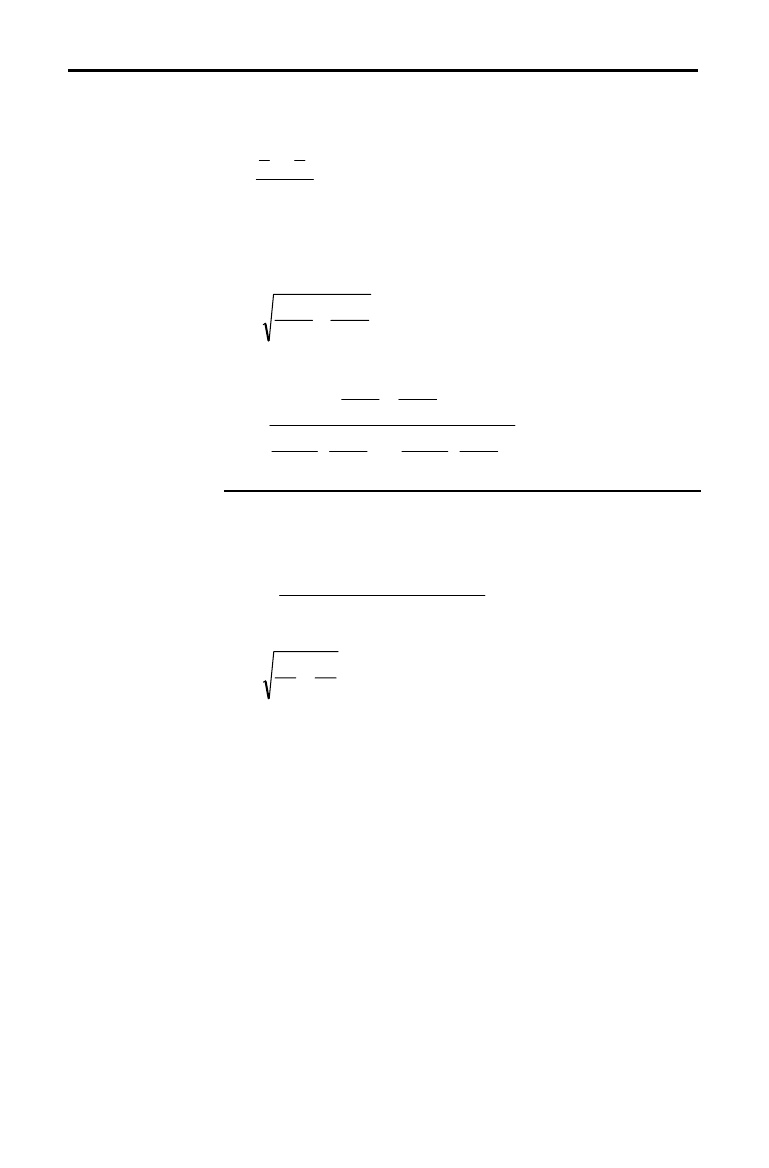
Tables and Reference Information A-53
8399APXA.DOC TI-83 international English Bob Fedorisko Revised: 02/19/01 1:25 PM Printed: 02/19/01 1:40 PM
Page 53 of 58
The following is the definition for the 2
.
SampTTest. The
two-sample
t
statistic with degrees of freedom
df
is:
t
xx
S
=
−
12
where the computation of
S
and
df
are dependent on
whether the variances are pooled. If the variances are not
pooled:
S
Sx
n
Sx
n
=+
1
2
1
2
2
2
df
Sx
n
Sx
n
n
Sx
nn
Sx
n
=
+
−
+
−
1
2
1
2
2
2
2
1
1
2
1
2
2
2
2
2
2
1
1
1
1
otherwise:
Sx
nSxnSx
df
p
=
−+−() ()
11
2
22
2
11
S
nn
Sx
p
=+
11
12
df n n
=+−
12
2
and
Sxp
is the pooled variance.
2-SampTTest

A-54 Tables and Reference Information
8399APXA.DOC TI-83 international English Bob Fedorisko Revised: 02/19/01 1:25 PM Printed: 02/19/01 1:40 PM
Page 54 of 58
This section contains financial formulas for computing time value of money,
amortization, cash flow, interest-rate conversions, and days between dates.
[]
ie
yx
=−
×+
(())
ln
1
1
where:
PMT ƒ
0
y
=
C/Y
÷
P/Y
x
= (.01
×
I%
)
÷
C/Y
C/Y
= compounding periods per year
P/Y
= payment periods per year
I%
= interest rate per year
iFVPV
N
=÷ −
−÷
()
()1
1
where:
PMT
=0
The iteration used to compute
i
:
0
11
1
=+ ×
−+
+×+
−
−
PV PMT G
i
i
FV i
i
N
N
()
()
[]
ICYe
yx
%/
=× × −
×+
1100
(ln( ))1
1
where:
x=i
y = P/Y
÷
C/Y
Gik
i
=+×
1
where:
k=
0 for end-of-period payments
k=
1 for beginning-of-period payments
N
PMT G FV i
PMT G PV i
i
i
i
=
×− ×
××
+
+
ln
ln
()1
where:
i ƒ
0
NPVFVPMT
=+÷
−
()
where:
i=
0
Financial Formulas
Time Value of
Money

Tables and Reference Information A-55
8399APXA.DOC TI-83 international English Bob Fedorisko Revised: 02/19/01 1:25 PM Printed: 02/19/01 1:40 PM
Page 55 of 58
PMT
i
G
PV
PV FV
i
i
N
=× +
+
+−
−
()11
where:
i ƒ
0
PMT PV FV N
=+÷
−
()
where:
i=
0
PV
PMT G
i
FV
i
PMT G
i
i
N
i
=
×
−
×
+
−
×1
1()
where:
i ƒ
0
PV FV PMT N
=+×
−
()
where:
i=
0
FV
PMT G
i
iPV
PMT G
i
i
N
i
=
×
−+ × +
×
()
1
where:
i ƒ
0
FV PV PMT N
=+×
−
()
where:
i
=0

A-56 Tables and Reference Information
8399APXA.DOC TI-83 international English Bob Fedorisko Revised: 02/19/01 1:25 PM Printed: 02/19/01 1:40 PM
Page 56 of 58
If computing
bal
(),
pmt
2 =
npmt
Let
bal
(0) =
RND
(
PV
)
Iterate from
m
= 1 to
pmt
2
I
I
m
m
=×−
=−−+
−
RND RND i bal m
bal m bal m RND PMT
[(())]
() ( ) ( )
12 1
1
then:
bal bal pmt
() ( )= 2
Σ
Pr n bal pmt bal pmt
() ( ) ( )
=−
21
ΣΣ
Int pmt pmt RND PMT n
() ( ) ( ) ()=−+× −211
Pr
where:
RND
= round the display to the number of
decimal places selected
RND12
= round to 12 decimal places
Balance, principal, and interest are dependent on the
values of
PMT, PV,
æ
, and
pmt
1 and
pmt
2.
Amortization

Tables and Reference Information A-57
8399APXA.DOC TI-83 international English Bob Fedorisko Revised: 02/19/01 1:25 PM Printed: 02/19/01 1:40 PM
Page 57 of 58
npv CF CF i
i
i
j
S
n
j
N
j
j
() ( )
(( ))
=+ +
−+
−
−
−
=
∑
0
1
1
11
1
where:
S
nj
j
j
i
i
j
=
≥
=
=
∑
1
1
00
Net present value is dependent on the values of the initial
cash flow (
CF
0
), subsequent cash flows (
CFj
), frequency of
each cash flow (
nj
), and the specified interest rate (
i
).
irr
() = 100
×
i
, where
i
satisfies
npv
() = 0
Internal rate of return is dependent on the values of the
initial cash flow (
CF
0
) and subsequent cash flows (
CFj
).
i
=
I
%
÷
100
4
Eff
() ( )
()
=× −
×+
100 1
1
e
CP xln
where:
x
= .01
×
NOM
÷
CP
[]
4
Nom
()
()
=×× −
÷× +
100 1
11
CP e
CP xln
where:
x
= .01
×
EFF
EFF
=
effective rate
CP
=
compounding periods
NOM
=
nominal rate
Cash Flow
Interest Rate
Conversions

A-58 Tables and Reference Information
8399APXA.DOC TI-83 international English Bob Fedorisko Revised: 02/19/01 1:25 PM Printed: 02/19/01 1:40 PM
Page 58 of 58
With the dbd( function, you can enter or compute a date
within the range Jan. 1, 1950, through Dec. 31, 2049.
Actual/actual day-count method (assumes actual
number of days per month and actual number of days per
year):
dbd
( (days between dates) =
Number of Days II
-
Number of Days I
Number of Days I = (
Y1
-
YB
)
×
365
+ (number of days
MB
to
M
1)
+
DT
1
+
()
YYB
1
4
−
Number of Days II = (
Y
2
-
YB
)
×
365
+ (number of days
MB
to
M
2)
+
DT
2
+
()
YYB
2
4
−
where:
M
1 = month of first date
DT
1 = day of first date
Y
1 = year of first date
M
2 = month of second date
DT
2 = day of second date
Y
2 = year of second date
MB
= base month (January)
DB
= base day (1)
YB
= base year (first year after leap year)
Days between
Dates

General Information B-1
8399APXB.DOC TI-83 Intl English, Appendix B Bob Fedorisko Revised: 02/19/01 1:12 PM Printed: 02/19/01 1:41
PM Page 1 of 14
B
General Information
Battery Information
......................................
B-2
In Case of Difficulty
.....................................
B-4
Error Conditions
.........................................
B-5
Accuracy Information
....................................
B-10
Support and Service Information
.........................
B-12
Warranty Information
....................................
B-13
Contents
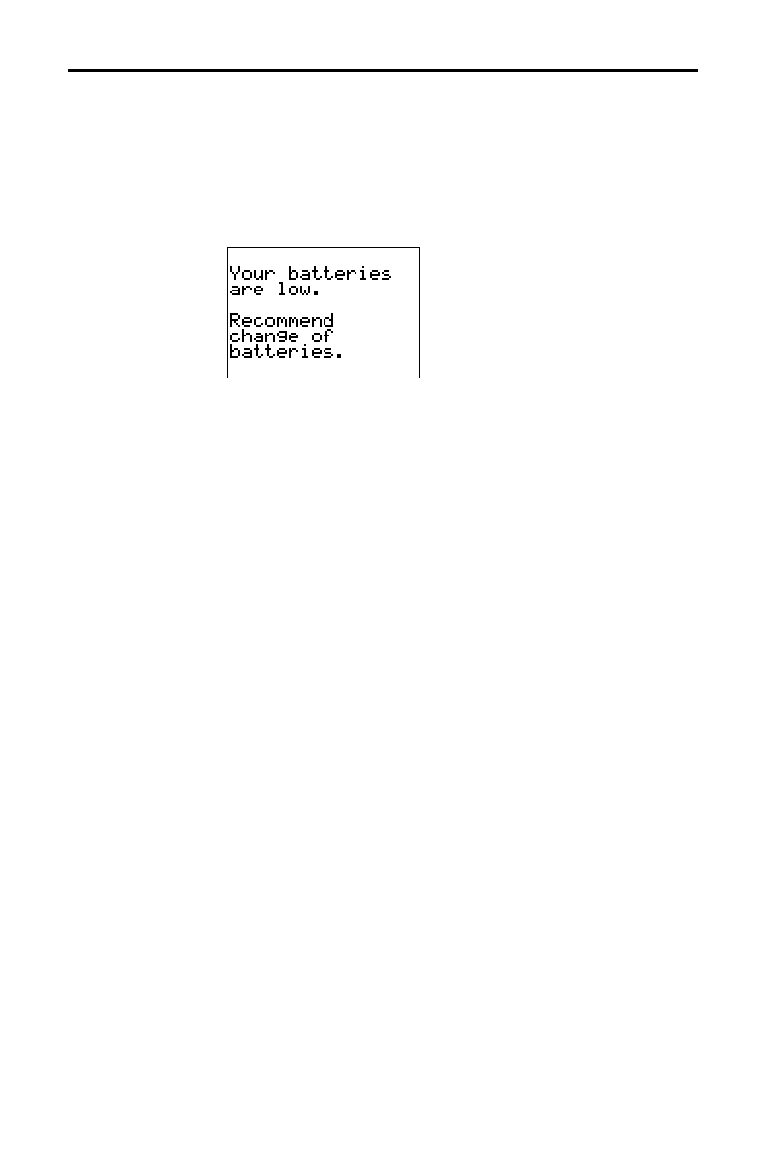
B-2 General Information
8399APXB.DOC TI-83 Intl English, Appendix B Bob Fedorisko Revised: 02/19/01 1:12 PM Printed: 02/19/01 1:41
PM Page 2 of 14
The TI
.
83 uses five batteries: four AAA alkaline batteries
and one lithium battery. The lithium battery provides
auxiliary power to retain memory while you replace the
AAA batteries.
When the battery voltage level drops below a usable level,
the TI
.
83 displays this message when you turn on the unit.
After this message is first displayed, you can expect the
batteries to function for about one or two weeks,
depending on usage. (This one-week to two-week period is
based on tests with alkaline batteries; the performance of
other kinds of batteries may vary.)
The low-battery message continues to be displayed each
time you turn on the unit until you replace the batteries. If
you do not replace the batteries within about two weeks,
the calculator may turn off by itself or fail to turn on until
you install new batteries.
Replace the lithium battery every three or four years.
Do not remove both types of batteries (AAA and lithium
auxiliary) at the same time. Do not allow the batteries to
lose power completely. If you follow these guidelines and
the steps for replacing batteries on page B
.
3, you can
replace either type of battery without losing any
information in memory.
Take these precautions when replacing batteries.
•
Do not mix new and used batteries. Do not mix brands
(or types within brands) of batteries.
•
Do not mix rechargeable and nonrechargeable
batteries.
•
Install batteries according to polarity (+ and
N
)
diagrams.
•
Do not place nonrechargeable batteries in a battery
recharger.
•
Properly dispose of used batteries immediately. Do not
leave them within the reach of children.
•
Do not incinerate batteries.
Battery Information
When to Replace
the Batteries
Effects of
Replacing the
Batteries
Battery
Precautions

General Information B-3
8399APXB.DOC TI-83 Intl English, Appendix B Bob Fedorisko Revised: 02/19/01 1:12 PM Printed: 02/19/01 1:41
PM Page 3 of 14
To replace the batteries, follow these steps.
1. Turn off the calculator. Replace the slide cover over the
keyboard to avoid inadvertently turning on the
calculator. Turn the back of the calculator toward you.
2. Hold the calculator upright. Place your thumb on the
oval indentation on the battery cover. Push down and
toward you to slide the cover about ¼ inch (6 mm). Lift
off the cover to expose the battery compartment.
Note: To avoid loss of information stored in
memory, you must turn off the calculator. Do not
remove the AAA batteries and the lithium battery
simultaneously.
3. Replace all four AAA alkaline batteries at the same
time. Or, replace the lithium battery.
•
To replace the AAA alkaline batteries, remove all
four discharged AAA batteries and install new ones
according to the polarity (+ and
N
) diagrams in the
battery compartment.
•
To remove the lithium battery, place your index
finger on the battery. Insert the tip of a ball-point pen
(or similar instrument) under the battery at the small
opening provided in the battery compartment.
Carefully pry the battery upward, holding it with
your thumb and finger. (There is a spring that pushes
against the underside of the battery.)
•
Install the new battery, + side up, by inserting the
battery and gently snapping it in with your finger.
Use a CR1616 or CR1620 (or equivalent) lithium
battery.
4. Replace the battery compartment cover. Turn the
calculator on and adjust the display contrast, if
necessary (step 1; page B
.
4).
Replacing the
Batteries

B-4 General Information
8399APXB.DOC TI-83 Intl English, Appendix B Bob Fedorisko Revised: 02/19/01 1:12 PM Printed: 02/19/01 1:41
PM Page 4 of 14
To handle a difficulty, follow these steps.
1. If you cannot see anything on the screen, the contrast
may need to be adjusted.
To darken the screen, press and release
y
, and then
press and hold
}
until the display is sufficiently dark.
To lighten the screen, press and release
y
, and then
press and hold
†
until the display is sufficiently light.
2. If an error menu is displayed, follow the steps in
Chapter 1. Refer to pages B
.
5 through B
.
9 for details
about specific errors, if necessary.
3. If a checkerboard cursor (
#
) is displayed, then either
you have entered the maximum number of characters in
a prompt, or memory is full. If memory is full, press
y
[
MEM
] 2 to select 2:Delete, and then delete some items
from memory (Chapter 18).
4. If the busy indicator (dotted line) is displayed, a graph
or program has been paused; the TI
.
83 is waiting for
input. Press
Í
to continue or press
É
to break.
5. If the calculator does not seem to work at all, be sure
the batteries are fresh and that they are installed
properly. Refer to battery information on pages B
.
2 and
B
.
3.
In Case of Difficulty
Handling a
Difficulty

General Information B-5
8399APXB.DOC TI-83 Intl English, Appendix B Bob Fedorisko Revised: 02/19/01 1:12 PM Printed: 02/19/01 1:41
PM Page 5 of 14
When the TI
.
83 detects an error, it displays ERR:
message
and an error menu.
Chapter 1 describes the general steps for correcting errors. This table contains
each error type, possible causes, and suggestions for correction.
Error Type Possible Causes and Suggested Remedies
ARCHIVED VAR
A function or instruction is archived and therefore cannot
be executed or edited. Use the unarchive command to
unarchive the variable before using it.
ARGUMENT
A function or instruction does not have the correct number
of arguments. See Appendix A and the appropriate chapter.
BAD GUESS
¦
In a
CALC
operation, you specified a Guess that is not
between Left Bound and Right Bound.
¦
For the
solve( function or the equation solver, you
specified a
guess
that is not between
lower
and
upper
.
¦
Your guess and several points around it are undefined.
Examine a graph of the function. If the equation has a
solution, change the bounds and/or the initial guess.
BOUND
¦
In a
CALC
operation or with Select(
,
you defined
Left Bound > Right Bound.
¦
In
fMin(, fMax(, solve(, or the equation solver, you
entered
lower
‚
upper
.
BREAK
You pressed the
É
key to break execution of a program,
to halt a
DRAW
instruction, or to stop evaluation of an
expression.
DATA TYPE
You entered a value or variable that is the wrong data type.
¦
For a function
(
includin
g
implied multiplication
)
or an
instruction, you entered an ar
g
ument that is an invalid
data type, such as a complex number where a real
number is required. See Appendix A and the appropriate
chapter.
¦
In an editor, you entered a type that is not allowed, such
as a matrix entered as an element in the stat list editor.
See the appropriate chapter.
¦
You attempted to store to an incorrect data type, such as
a matrix, to a list.
DIM MISMATCH
You attempted to perform an operation that references
more than one list or matrix, but the dimensions do not
match.
DIVIDE BY 0
¦
You attempted to divide by zero. This error is not
returned durin
g
g
raphin
g
. The TI
.
83 allows for
undefined values on a graph.
¦
You attempted a linear regression with a vertical line.
Error Conditions

B-6 General Information
8399APXB.DOC TI-83 Intl English, Appendix B Bob Fedorisko Revised: 02/19/01 1:12 PM Printed: 02/19/01 1:41
PM Page 6 of 14
Error Type Possible Causes and Suggested Remedies
DOMAIN
¦
You specified an ar
g
ument to a function or instruction
outside the valid ran
g
e. This error is not returned durin
g
g
raphin
g
. The TI
.
83 allows for undefined values on a
graph. See Appendix A and the appropriate chapter.
¦
You attempted a lo
g
arithmic or power re
g
ression with a
L
X
or an exponential or power regression with a
L
Y
.
¦
You attempted to compute
G
Prn(
or
G
Int(
with
pmt2
<
pmt1
.
Duplicate Name
A variable you attempted to transmit cannot be transmitted
because a variable with that name already exists in the
receiving unit.
Error in Xmit
¦
The TI
.
83 was unable to transmit an item. Check to see
that the cable is firmly connected to both units and that
the receiving unit is in receive mode.
¦
You pressed
É
to break during transmission.
¦
You attempted to perform a backup from a TI
.
82 to a
TI
.
83.
¦
You attempted to transfer data
(
other than
L
1
throu
g
h
L
6
) from a TI
.
83 to a TI
.
82.
¦
You attempted to transfer
L
1
throu
g
h
L
6
from a TI
.
83 to
a TI
.
82 without usin
g
5:Lists to TI82
on the
LINK SEND
menu.
ILLEGAL NEST
You attempted to use an invalid function in an ar
g
ument to
a function, such as
seq(
within
expression
for
seq(
.
INCREMENT
¦
The increment in
seq(
is 0 or has the wron
g
si
g
n. This
error is not returned durin
g
g
raphin
g
. The TI
.
83 allows
for undefined values on a graph.
¦
The increment in a
For(
loop is 0.
INVALID
¦
You attempted to reference a variable or use a function
where it is not valid. For example,
Y
n
cannot reference
Y
,
Xmin
,
@
X
, or
TblStart
.
¦
You attempted to reference a variable or function that
was transferred from the TI
.
82 and is not valid for the
TI
.
83. For example, you may have transferred
U
n
N
1
to
the TI
.
83 from the TI
.
82 and then tried to reference it.
¦
In
Seq
mode, you attempted to
g
raph a phase plot
without defining both equations of the phase plot.

General Information B-7
8399APXB.DOC TI-83 Intl English, Appendix B Bob Fedorisko Revised: 02/19/01 1:12 PM Printed: 02/19/01 1:41
PM Page 7 of 14
Error Type Possible Causes and Suggested Remedies
INVALID (cont.)
¦
In
Seq
mode, you attempted to
g
raph a recursive
sequence without havin
g
input the correct number of
initial conditions.
¦
In
Seq
mode, you attempted to reference terms other
than
(
n
N
1)
or
(
n
N
2)
.
¦
You attempted to desi
g
nate a
g
raph style that is invalid
within the current graph mode.
¦
You attempted to use
Select(
without havin
g
selected
(turned on) at least one xyLine or scatter plot.
INVALID DIM
¦
You specified dimensions for an ar
g
ument that are not
appropriate for the operation.
¦
You specified a list dimension as somethin
g
other than
an integer between 1 and 999.
¦
You specified a matrix dimension as somethin
g
other
than an integer between 1 and 99.
¦
You attempted to invert a matrix that is not square.
ITERATIONS
¦
The
solve(
function or the equation solver has exceeded
the maximum number of permitted iterations. Examine
a
g
raph of the function. If the equation has a solution,
change the bounds, or the initial guess, or both.
¦
irr(
has exceeded the maximum number of permitted
iterations.
¦
When computin
g
æ
, the maximum number of iterations
was exceeded.
LABEL
The label in the
Goto
instruction is not defined with a
Lbl
instruction in the program.
MEMORY
Memory is insufficient to perform the instruction or
function. You must delete items from memory
(
Chapter 18
)
before executing the instruction or function.
Recursive problems return this error; for example,
graphing the equation
Y
1
=Y
1
.
Branchin
g
out of an
If
/
Then
,
For(
,
While
, or
Repeat
loop with
a
Goto
also can return this error because the
End
statement
that terminates the loop is never reached.

B-8 General Information
8399APXB.DOC TI-83 Intl English, Appendix B Bob Fedorisko Revised: 02/19/01 1:12 PM Printed: 02/19/01 1:41
PM Page 8 of 14
Error Type Possible Causes and Suggested Remedies
MemoryFull
¦
You are unable to transmit an item because the receivin
g
unit’s available memory is insufficient. You may skip the
item or exit receive mode.
¦
Durin
g
a memory backup, the receivin
g
unit’s available
memory is insufficient to receive all items in the sendin
g
unit’s memory. A messa
g
e indicates the number of bytes
the sendin
g
unit must delete to do the memory backup.
Delete items and try again.
MODE
You attempted to store to a window variable in another
g
raphin
g
mode or to perform an instruction while in the
wron
g
mode; for example,
DrawInv
in a
g
raphin
g
mode
other than
Func
.
NO SIGN CHNG
¦
The
solve(
function or the equation solver did not detect
a sign change.
¦
You attempted to compute
æ
when
FV
,
(
Úä
PMT
)
, and
PV
are all
‚
0, or when
FV
, (
Úä
PMT
), and
PV
are all
0.
¦
You attempted to compute
irr(
when neither
CFList
nor
CFO
is > 0, or when neither
CFList
nor
CFO
is < 0.
NONREAL ANS
In
Real
mode, the result of a calculation yielded a complex
result. This error is not returned durin
g
g
raphin
g
. The TI
.
83
allows for undefined values on a graph.
OVERFLOW
You attempted to enter, or you have calculated, a number
that is beyond the ran
g
e of the calculator. This error is not
returned durin
g
g
raphin
g
. The TI
.
83 allows for undefined
v
alues on a graph.
RESERVED
You attempted to use a system variable inappropriately.
See Appendix A.
SINGULAR MAT
¦
A sin
g
ular matrix
(
determinant = 0
)
is not valid as the
argument for
L
1
.
¦
The
SinReg
instruction or a polynomial re
g
ression
g
enerated a sin
g
ular matrix
(
determinant = 0
)
because it
could not find a solution, or a solution does not exist.
This error is not returned durin
g
g
raphin
g
. The TI
.
83
allows for undefined values on a graph.

General Information B-9
8399APXB.DOC TI-83 Intl English, Appendix B Bob Fedorisko Revised: 02/19/01 1:12 PM Printed: 02/19/01 1:41
PM Page 9 of 14
Error Type Possible Causes and Suggested Remedies
SINGULARITY
expression
in the
solve(
function or the equation solver
contains a sin
g
ularity
(
a point at which the function is not
defined
)
. Examine a
g
raph of the function. If the equation
has a solution, chan
g
e the bounds or the initial
g
uess or
both.
STAT
You attempted a stat calculation with lists that are not
appropriate.
¦
Statistical analyses must have at least two data points.
¦
Med
.
Med
must have at least three points in each
partition.
¦
When you use a
frequency list, its elements must be
‚
0.
¦
(
Xmax
N
Xmin
)
à
Xscl
must be
47 for a histogram.
STAT PLOT
You attempted to display a
g
raph when a stat plot that uses
an undefined list is turned on.
SYNTAX
The command contains a syntax error. Look for misplaced
functions, ar
g
uments, parentheses, or commas. See
Appendix A and the appropriate chapter.
TOL NOT MET
You requested a tolerance to which the al
g
orithm cannot
return an accurate result.
UNDEFINED
You referenced a variable that is not currently defined. For
example, you referenced a stat variable when there is no
current calculation because a list has been edited, or you
referenced a variable when the variable is not valid for the
current calculation, such as
a
after
Med
.
Med
.
WINDOW RANGE
A problem exists with the window variables.
¦
You defined
Xmax
Xmin
or
Ymax
Ymin
.
¦
You defined
q
max
q
min
and
q
step
>
0
(or vice versa).
¦
You attempted to define
Tstep=0
.
¦
You defined
Tmax
Tmin
and
Tstep
>
0
(or vice versa).
¦
Window variables are too small or too lar
g
e to
g
raph
correctly. You may have attempted to zoom in or zoom
out to a point that exceeds the TI
.
83’s numerical range.
ZOOM
¦
A point or a line, instead of a box, is defined in
ZBox.
¦
A
ZOOM
operation returned a math error.

B-10 General Information
8399APXB.DOC TI-83 Intl English, Appendix B Bob Fedorisko Revised: 02/19/01 1:12 PM Printed: 02/19/01 1:41
PM Page 10 of 14
To maximize accuracy, the TI
.
83 carries more digits
internally than it displays. Values are stored in memory
using up to 14 digits with a two-digit exponent.
•
You can store a value in the window variables using up
to 10 digits (12 for
Xscl, Yscl, Tstep, and
q
step
).
•
Displayed values are rounded as specified by the mode
setting with a maximum of 10 digits and a two-digit
exponent.
•
RegEQ displays up to 14 digits in Float mode. Using a
fixed-decimal setting other than Float causes RegEQ
results to be rounded and stored with the specified
number of decimal places.
Xmin is the center of the leftmost pixel, Xmax is the center
of the next-to-the-rightmost pixel. (The rightmost pixel is
reserved for the busy indicator.)
@
X
is the distance
between the centers of two adjacent pixels.
•
In
Full screen mode,
@
X is calculated as
(Xmax
N
Xmin)
à
94. In G
.
T split-screen mode,
@
X
is
calculated as (Xmax
N
Xmin)
à
46.
•
If you enter a value for
@
X
from the home screen or a
program in Full screen mode, Xmax is calculated as
Xmin +
@
X
…
94. In G
.
T split-screen mode, Xmax is
calculated as Xmin +
@
X
…
46.
Ymin is the center of the next-to-the-bottom pixel; Ymax is
the center of the top pixel.
@
Y
is the distance between the
centers of two adjacent pixels.
•
In
Full screen mode,
@
Y
is calculated as
(Ymax
N
Ymin)
à
62. In Horiz split-screen mode,
@
Y
is
calculated as (Ymax
N
Ymin)
à
30. In G
.
T split-screen
mode,
@
Y
is calculated as (Ymax
N
Ymin)
à
50.
•
If you enter a value for
@
Y
from the home screen or a
program in Full screen mode, Ymax is calculated as
Ymin +
@
Y
…
62. In Horiz split-screen mode, Ymax is
calculated as Ymin +
@
Y
…
30. In G
.
T split-screen mode,
Ymax is calculated as Ymin +
@
Y
…
50.
Accuracy Information
Computational
Accuracy
Graphing
Accuracy

General Information B-11
8399APXB.DOC TI-83 Intl English, Appendix B Bob Fedorisko Revised: 02/19/01 1:12 PM Printed: 02/19/01 1:41
PM Page 11 of 14
Cursor coordinates are displayed as eight-character
numbers (which may include a negative sign, decimal
point, and exponent) when
Float mode is selected. X and Y
are updated with a maximum accuracy of eight digits.
minimum and maximum on the
CALCULATE
menu are
calculated with a tolerance of 1
E
L
5;
‰
f(x)dx
is calculated at
1
E
L
3. Therefore, the result displayed may not be accurate to
all eight displayed digits. For most functions, at least five
accurate digits exist. For
fMin(, fMax(, and fnInt( on the
MATH
menu and solve( in the
CATALOG
, the tolerance can
be specified.
Function Range of Input Values
sin
x
, cos
x
, tan
x
0
|
x
| < 10
12
(radian or degree)
sin
L
1
x
, cos
L
1
x
L
1
x
1
ln
x
, log
x
10
L
100
<
x
< 10
100
e
x
L
10
100
<
x
230.25850929940
10
x
L
10
100
<
x
< 100
sinh
x
, cosh
x
|
x
|
230.25850929940
tanh
x
|
x
| < 10
100
sinh
L
1
x
|
x
| < 5 × 10
99
cosh
L
1
x
1
x
< 5 × 10
99
tanh
L
1
x
L
1 <
x
< 1
‡
x
(real mode) 0
x
< 10
100
‡
x
(complex mode) |
x
| < 10
100
x
!
L
.5
x
69, where
x
is a multiple of .5
Function Range of Result
sin
L
1
x
, tan
L
1
x
L
90
¡
to 90
¡
or
Lpà
2 to
pà
2 (radians)
cos
L
1
x
0
¡
to 180
¡
or 0 to
p
(radians)
Function Limits
Function Results

B-12 General Information
8399APXB.DOC TI-83 Intl English, Appendix B Bob Fedorisko Revised: 02/19/01 1:12 PM Printed: 02/19/01 1:41
PM Page 12 of 14
Product Support
Customers in the U.S., Canada, Puerto Rico, and the Virgin Islands
For general questions, contact Texas Instruments Customer Support:
phone:
1
.
800
.
TI
.
CARES (1
.
800
.
842
.
2737)
e-mail: [email protected]
For technical questions, call the Programming Assistance Group of Customer
Support:
phone:
1
.
972
.
917
.
8324
Customers outside the U.S., Canada, Puerto Rico, and the Virgin Islands
Contact TI by e-mail or visit the TI calculator home page on the World Wide Web.
e-mail:
Internet: education.ti.com
Product Service
Customers in the U.S. and Canada Only
A
lways contact Texas Instruments Customer Support before returning a product
for service.
Customers outside the U.S. and Canada
Refer to the leaflet enclosed with this product or contact your local Texas
Instruments retailer/distributor.
Other TI Products and Services
V
isit the TI calculator home page on the World Wide Web.
education.ti.com
Refer to the leaflet enclosed with this product or contact your local Texas
Instruments retailer/distributor.
Support and Service Information

General Information B-13
8299APPB.DOC TI-82, Appendix B, English Bob Fedorisko Revised: 02/27/01 12:20 PM Printed:
02/27/01 12:25 PM Page 12 of 13
Warranty Information
Customers in the U.S. and Canada Only
One-Year Limited Warranty for Electronic Product
This Texas Instruments (“TI”) electronic product warranty extends only to the original
purchaser and user of the product.
Warranty Duration.
This TI electronic product is warranted to the original purchaser
for a period of one (1) year from the original purchase date.
Warranty Coverage.
This TI electronic product is warranted against defective
materials and construction.
THIS WARRANTY IS VOID IF THE PRODUCT HAS BEEN
DAMAGED BY ACCIDENT OR UNREASONABLE USE, NEGLECT, IMPROPER
SERVICE, OR OTHER CAUSES NOT ARISING OUT OF DEFECTS IN MATERIALS
OR CONSTRUCTION.
Warranty Disclaimers.
ANY IMPLIED WARRANTIES ARISING OUT OF THIS SALE,
INCLUDING BUT NOT LIMITED TO THE IMPLIED WARRANTIES OF
MERCHANTABILITY AND FITNESS FOR A PARTICULAR PURPOSE, ARE LIMITED
IN DURATION TO THE ABOVE ONE-YEAR PERIOD. TEXAS INSTRUMENTS SHALL
NOT BE LIABLE FOR LOSS OF USE OF THE PRODUCT OR OTHER INCIDENTAL
OR CONSEQUENTIAL COSTS, EXPENSES, OR DAMAGES INCURRED BY THE
CONSUMER OR ANY OTHER USER.
Some states/provinces do not allow the exclusion or limitation of implied warranties or
consequential damages, so the above limitations or exclusions may not apply to you.
Legal Remedies.
This warranty gives you specific legal rights, and you may also have
other rights that vary from state to state or province to province.
Warranty Performance.
During the above one (1) year warranty period, your defective
product will be either repaired or replaced with a reconditioned model of an equivalent
quality (at TI’s option) when the product is returned, postage prepaid, to Texas
Instruments Service Facility. The warranty of the repaired or replacement unit will
continue for the warranty of the original unit or six (6) months, whichever is longer.
Other than the postage requirement, no charge will be made for such repair and/or
replacement. TI strongly recommends that you insure the product for value prior to
mailing.
Software.
Software is licensed, not sold. TI and its licensors do not warrant that the
software will be free from errors or meet your specific requirements.
All software is
provided “AS IS.”
Copyright.
The software and any documentation supplied with this product are
protected by copyright.

B-14 General Information
8299APPB.DOC TI-82, Appendix B, English Bob Fedorisko Revised: 02/27/01 12:20 PM Printed:
02/27/01 12:25 PM Page 13 of 13
Australia & New Zealand Customers only
One-Year Limited Warranty for Commercial Electronic Product
This Texas Instruments electronic product warranty extends only to the
original purchaser and user of the product.
Warranty Duration.
This Texas Instruments electronic product is warranted
to the original purchaser for a period of one (1) year from the original
purchase date.
Warranty Coverage.
This Texas Instruments electronic product is warranted
against defective materials and construction. This warranty is void if the
product has been damaged by accident or unreasonable use, neglect, improper
service, or other causes not arising out of defects in materials or construction.
Warranty Disclaimers. Any implied warranties arising out of this sale,
including but not limited to the implied warranties of merchantability
and fitness for a particular purpose, are limited in duration to the
above one-year period. Texas Instruments shall not be liable for loss
of use of the product or other incidental or consequential costs,
expenses, or damages incurred by the consumer or any other user.
Some jurisdictions do not allow the exclusion or limitation of implied
warranties or consequential damages, so the above limitations or exclusions
may not apply to you.
Legal Remedies. This warranty gives you specific legal rights, and you may
also have other rights that vary from jurisdiction to jurisdiction.
Warranty Performance.
During the above one (1) year warranty period,
your defective product will be either repaired or replaced with a new or
reconditioned model of an equivalent quality (at TI’s option) when the product
is returned to the original point of purchase. The repaired or replacement unit
will continue for the warranty of the original unit or six (6) months, whichever
is longer. Other than your cost to return the product, no charge will be made
for such repair and/or replacement. TI strongly recommends that you insure
the product for value if you mail it.
Software.
Software is licensed, not sold. TI and its licensors do not warrant
that the software will be free from errors or meet your specific requirements.
All software is provided “AS IS.”
Copyright.
The software and any documentation supplied with this product
are protected by copyright.
All Customers Outside the U.S. and Canada
For information about the length and terms of the warranty, refer to your package
and/or to the warranty statement enclosed with this product, or contact your local Texas
Instruments retailer/distributor.

Index-1
Index
8399INDX.DOC TI-83 international English Bob Fedorisko Revised: 02/20/01 10:54 AM Printed: 02/21/01 8:40
AM Page 1 of 16
+
(addition),
2-3
,
A-38
c
2
cdf(
(chi-square cdf),
13-31
,
A-3
c
2
pdf(
(chi-square pdf),
13-31
,
A-4
c
2
.
Test
(chi-square test),
13-22
,
A-4
:
(colon),
6, 16-5
+
(concatenation),
15-6
,
A-38
3
(cube),
2-6, A-35
3
‡
(
(cube root),
2-6, A-35
¡
(degrees notation),
2-3
,
A-34
à
(division),
2-3, A-37
=
(equal-to relational test),
2-25,
A-35
!
(factorial),
2-21
,
A-34
ì
(graph style, animate),
3-9
í
(graph style, dot),
3-9
ç
(graph style, line),
3-9
>
(greater than),
2-25, A-35
‚
(greater than or equal to),
2-25,
A-35
L
1
(inverse),
2-3
,
8-9
,
10-10, A-36
<
(less than),
2-25, A-35
(less than or equal to),
2-25, A-36
{ }
(list indicator),
11-4
[ ]
(matrix indicator),
10-7
'
(minutes notation),
2-23, A-38
ä
(multiplication),
2-3, A-37
M
(negation),
1-23, 2-4, A-37
ƒ
(not equal to),
2-25, A-35
( )
(parentheses),
1-23
p
(pi),
2-4
›
(pixel mark),
8-15, 12-34
+
(pixel mark),
8-15, 12-34
¦
(pixel mark),
8-15, 12-34
Ö
(plot type, box),
12-33
Ò
(plot type, histogram),
12-32
Õ
(plot type, modified box),
12-32
Ô
(plot type, normal probability),
12-33
^
(power),
2-3
,
A-36
,
A-37
10
^(
(power of ten),
2-4
,
A-37
x
‡
(root),
2-6, A-35
"
(seconds notation),
2-23, A-38
2
(square) ,
2 - 3 , A-36
‡
(
(square root) ,
2 - 3 , A-37
!
Store,
1-14, A-28
" "
(string indicator),
15-3
N
(subtraction),
2-3, A-38
.
A
.
a+b
i
(rectangular complex mode),
1-12, 2-16
,
A-3
above graph style(
é
),
3-9
abs(
(absolute value),
2-13
,
2-19
,
10-10
,
A-2
accuracy information
computational and graphing,
B-10
graphing,
3-17
function limits and results,
B-11
addition (
+
),
2-3
,
A-38
alpha cursor,
1-5
alpha key,
3
alpha-lock,
1-8
alternative hypothesis,
13-7
amortization
bal(
(amortization balance),
14-9
,
A-3
calculating schedules,
14-9
formula,
A-56
G
Int(
(sum of interest),
14
.
9
,
A-12
G
Prn(
(sum of principal),
14-9
,
A-19
and
(Boolean operator),
2-26
,
A-2
angle(
,
2-19
,
A-2
ANGLE
menu,
2-23
angle modes,
1-11
animate graph style (
ì
),
3-9
ANOVA(
(one-way variance analysis),
13-25
,
A-2
formula,
A-51
Ans
(last answer),
1-18
,
A-2
APD
é
(Automatic Power Down™),
1-2
applications.
See
examples,
applications
arccosine (
cos
M
1
(
),
2-3
arcsine (
sin
M
1
(
),
2-3
arctangent (
tan
M
1
(
),
2-3
augment(
,
10-14
,
11-15
,
A-3
Automatic Power Down™ (APD
é
),
1-2
automatic regression equation,
12-22
automatic residual list (
RESID
),
12-22
axes format, sequence graphing,
6-8
axes, displaying (
AxesOn
,
AxesOff
),
3-14
,
A-3
AxesOff
,
3-14
,
A-3
AxesOn
,
3-14
,
A-3

Index-2
8399INDX.DOC TI-83 international English Bob Fedorisko Revised: 02/20/01 10:54 AM Printed: 02/21/01 8:40
AM Page 2 of 16
.
B
.
backing up calculator memory,
19-4,
19-10
bal(
(amortization balance),
14-9
,
A-3
batteries,
1-2
,
B-2
below graph style (
ê
),
3-9
binomcdf(
,
13-33
,
A-3
binompdf(
,
13-33
,
A-3
Boolean logic,
2-26
box pixel mark (
›
),
8-15, 12-34
Boxplot
plot type (
Ö
),
12-33
busy indicator,
1-4
.
C
.
CALCULATE
menu,
3-25
Calculate
output option,
13-6, 13-8
cash flow
calculating,
14-8
formula,
A-57
irr(
(internal rate of return),
14-8
,
A-13
npv(
(net present value),
14-8
,
A-17
CATALOG
,
15-2
CBL 2/CBL System,
16-21, 19-3
,
A-10
CBR,
16-21, 19-3
,
A-10
Check RAM
(memory screen),
18-2
chi-square cdf (
c
2
cdf(
),
13-31
,
A-3
chi-square pdf (
c
2
pdf(
),
13-31
,
A-4
chi-square test (
c
2
.
Test
),
13-22
,
A-4
Circle(
(draw circle),
8-11
,
A-4
Clear Entries
,
18-4
,
A-4
clearing
entries (
Clear Entries
),
18-4
,
A-4
all lists (
ClrAllLists
),
18-4
,
A-4
drawing (
ClrDraw
),
8-4
,
A-4
home screen (
ClrHome
),
16-20
,
A-4
list (
ClrList
),
12-20
,
A-4
table (
ClrTable
),
16-20
,
A-4
ClrAllLists
(clear all lists),
18-4
,
A-4
ClrDraw
(clear drawing),
8-4
,
A-4
ClrHome
(clear home screen),
16-20
,
A-4
ClrList
(clear list),
12-20
,
A-4
ClrTable
(clear table),
16-20
,
A-4
coefficients of determination (
r
2
,
R
2
),
12-23
colon separator (
:
),
6, 16-5
combinations (
nCr
),
2-21
,
A-16
.
C (continued)
.
complex
modes (
a+b
i
,
r
e
^
q
i
),
1-12, 2-16
,
A-3
,
A-22
numbers,
1-12
,
2-16
,
2-18
,
A-22
compounding-periods-per-year variable
(
C/Y
),
14-4, 14-14
concatenation (
+
),
15-6
,
A-38
confidence intervals,
13-8, 13-16
N
13
.
21
conj(
(conjugate),
2-18
,
A-4
Connected
(plotting mode),
1-11
,
A-4
contrast (display),
1-3
convergence, sequence graphing,
6-12
conversions
4
Dec
(to decimal),
2-5
,
A-5
4
DMS
(to degrees/minutes/ seconds),
2-24, A-7
4
Eff
(to effective interest rate),
14-12, A-7
Equ
4
String(
(equation-to-string
conversion),
15-7, A-8
4
Frac
(to fraction conversion),
2-5,
A-10
List
4
matr(
(list-to-matrix
conversion),
10-14, 11-15, A-14
Matr
4
list(
(matrix-to-list conversion),
10-14, 11-16, A-15
4
Nom
(to nominal interest rate
conversion),
14-12, A-16
4
Polar
(to polar conversion),
2-19,
A-19
P
4
Rx(
,
P
4
Ry(
(polar-to-rectangular
conversion),
2-24, A-21
4
Rect
(to rectangular conversion),
2-19, A-22
R
4
Pr(
,
R
4
P
q
(
(rectangular-to-polar
conversion),
2-24, A-23
String
4
Equ(
(string-to-equation
conversion),
15-8, A-29
CoordOff
,
3-14, A-5
CoordOn
,
3-14, A-5
correlation coefficient (
r
),
12-23, 12-25
to
12
-
27
cos(
(cosine),
2-3, A-5
cos
M
1
(
(arccosine),
2-3, A-5
cosh(
(hyperbolic cosine),
15-10, A-5

Index-3
8399INDX.DOC TI-83 international English Bob Fedorisko Revised: 02/20/01 10:54 AM Printed: 02/21/01 8:40
AM Page 3 of 16
.
D (continued)
.
cosh
M
1
(
(hyperbolic arccosine),
15-10,
A-5
cosine (
cos(
),
2-3, A-5
cross pixel mark (
+
),
8-15, 12-34
cube (
3
),
2-6, A-35
cube root (
3
‡
(
),
2-6, A-35
CubicReg
(cubic regression),
12-26,
A-5
cubic regression (
CubicReg
),
12-26,
A-5
cumulative sum (
cumSum(
),
10-15
,
11-12, A-5
cumSum(
(cumulative sum),
10-15
,
11-12, A-5
cursors,
1-5
,
1-8
C/Y
(compounding-periods-per-year
variable),
14-4, 14-14
.
D
.
Data input option,
13-6, 13-7
days between dates (
dbd(
),
14-13, A-5,
A-58
dbd(
(days between dates),
14-13, A-5,
A-58
4
Dec
(to decimal conversion),
2-5, A-5
decimal mode (float or fixed),
1-10
decrement and skip (
DS<(
),
16-14, A-7
definite integral,
2-7, 3-28, 4-8, 5-6
Degree
angle mode,
1-11
,
2-23, A-6
degrees notation (
¡
),
2-3
,
A-34
DELETE FROM
menu,
18-3
delete variable contents (
DelVar
),
16-15, A-6
DelVar
(delete variable contents),
16-15, A-6
DependAsk
,
7-3, 7-5, A-6
DependAuto
,
7-3, 7-5, A-6
derivative.
See
numerical derivative
det(
(determinant),
10-12, A-6
determinant (
det(
),
10-12, A-6
DiagnosticOff
,
12-23, A-6
DiagnosticOn
,
12-23, A-6
diagnostics display mode(
r
,
r
2
,
R
2
),
12-23
differentiation,
2-8, 3-28, 4-8, 5-6
.
D (continued)
.
dimensioning a list or matrix,
10-12
,
10-13
,
11-11, A-6
dim(
(dimension),
10-12
,
11-11, A-6
!
dim(
(assign dimension),
10-13
,
11-11, A-6
Disp
(display),
16-18, A-6
DispGraph
(display graph),
16-19, A-7
display contrast,
1-3
display cursors,
1-5
DispTable
(display table),
16-19, A-7
DISTR
(distributions menu),
13-29
DISTR DRAW
(distributions drawing
menu),
13-35
distribution functions
binomcdf(
,
13-33, A-3
binompdf(
,
13-33, A-3
c
2
cdf(
,
13-31, A-3
c
2
pdf(
,
13-31, A-4
Û
cdf(
,
13-32, A-8
Û
pdf(
,
13-32, A-9
geometcdf(
,
13-34, A-10
geometpdf(
,
13-34, A-11
invNorm(
,
13-30, A-12
normalcdf(
,
13-30, A-17
normalpdf(
,
13-29, A-17
poissoncdf(
,
13-34, A-99
poissonpdf(
,
13-33, A-19
tcdf(
,
13-31, A-29
tpdf(
,
13-30, A-29
distribution shading instructions
Shade
c
2
(
,
13-36, A-26
Shade
Û
(
,
13-36, A-27
ShadeNorm(
,
13-35, A-27
Shade_t(
,
13-36, A-27
division (
à
),
2-3, A-37
DMS (degrees/minutes/seconds entry
notation),
2-23, A-38
4
DMS
(to degrees/minutes/seconds),
2-24, A-7
dot graph style (
í
),
3-9
dot pixel mark (
¦
),
8-15, 12-34
Dot
(plotting mode),
1-11, A-7
DrawF
(draw a function),
8-9, A-7

Index-4
8399INDX.DOC TI-83 international English Bob Fedorisko Revised: 02/20/01 10:54 AM Printed: 02/21/01 8:40
AM Page 4 of 16
.
D (continued)
.
drawing on a graph
circles (
Circle(
),
8-11
functions and inverses (
DrawF
,
DrawInv
),
8-9
lines (
Horizontal
,
Line(
,
Vertical
),
8-6, 8-7
line segments (
Line(
),
8-5
pixels (
Pxl
.
Change
,
Pxl
.
Off
,
Pxl
.
On
,
pxl
.
Test
),
8-16
points (
Pt
.
Change
,
Pt
.
Off
,
Pt
.
On
),
8-14
tangents (
Tangent
),
8-8
text (
Text
),
8-12
using
Pen
,
8-13
DrawInv
(draw inverse),
8-9, A-7
DRAW
menu,
8-3
DRAW
instructions,
8-3
N
8
.
16
Draw output option,
13-6
N
13
.
8
DRAW POINTS
menu,
8-14
DRAW STO
(draw store menu),
8-17
dr/d
q
operation on a graph,
5-6
DS<(
(decrement and skip),
16-14, A-7
DuplicateName
menu,
19-5
dx/dt
operation on a graph,
3-28, 4-8
dy/dx
operation on a graph,
3-28, 4-8,
5-6
.
E
.
e
(constant)
, 2-4
e^(
(exponential),
2-4, A-7
å (exponent),
1-7, 1-10, A-7
edit keys table,
1-8
4
Eff(
(to effective interest rate),
14-12,
A-7
Else
,
16-10
End
,
16-12, A-8
Eng
(engineering notation mode),
1-10,
A-8
entry cursor,
1-5
ENTRY
(last entry key),
1-16
EOS
é
(Equation Operating System),
1-22
eqn
(equation variable),
2-8, 2-12
equal-to relational test (
=
),
2-25, A-35
Equation Operating System (EOS
é
),
1-22
Equation Solver
,
2-8
equations with multiple roots,
2-12
.
E (continued)
.
Equ
4
String(
(equation-to-string
conversion),
15-7, A-8
errors
diagnosing and correcting,
1-24
messages,
B-5
examples—applications
area between curves,
17-11
areas of regular n-sided polygons,
17-16
box plots,
17-2
cobweb attractors,
17-8
fundamental theorem of calculus,
17-14
guess the coefficients,
17-9
inequalities,
17-5
mortgage payments
17
.
18
parametric equations: ferris wheel
problem,
17-12
piecewise functions,
17-4
Sierpinski triangle,
17-7
solving a system of nonlinear
equations,
17-6
unit circle and trig curves,
17-10
examples—Getting Started
box with lid
9 to 16
defining a,
9
defining a table of values,
10
finding calculated maximum,
16
setting the viewing window,
12
tracing the graph,
13
zooming in on the graph,
15
zooming in on the table,
11
coin flip,
2-2
compound interest,
14-3
drawing a tangent line,
8-2
financing a car,
14-2
forest and trees,
6-2
generating a sequence,
11-2
graphing a circle,
3-2
mean height of a population,
13-2
path of a ball,
4-2
pendulum lengths and periods,
12-2
polar rose,
5-2

Index-5
8399INDX.DOC TI-83 international English Bob Fedorisko Revised: 02/20/01 10:54 AM Printed: 02/21/01 8:40
AM Page 5 of 16
.
E (continued)
.
examples—Getting Started (continued)
quadratic formula
converting to a fraction,
7
displaying complex results,
8
entering a calculation,
6
roots of a,
7-2
sending variables,
19-2
solving a system of linear equations,
10-2
unit circle,
9-2
volume of a cylinder,
16-2
examples—miscellaneous
convergence,
6-12
daylight hours in Alaska,
12-28
calculating outstanding loan
balances,
14-10
predator-prey model,
6-13
exponential regression (
ExpReg
),
12-26, A-8
expr(
(string-to-expression conversion),
15-7, A-8
ExpReg
(exponential regression),
12-26, A-8
expression,
1-6
converting from string (
expr(
),
15-7,
A-8
turning on and off (
ExprOn
,
ExprOff
),
3-14, A-8
ExprOff
(expression off),
3-14, A-8
ExprOn
(expression on),
3-14, A-8
.
F
.
‰
f(x)dx
operation on a graph,
3-28
factorial (
!
),
2-21
,
A-34
family of curves,
3-16
Û
cdf(
,
13-32, A-8
Fill(
,
10-13, A-8
FINANCE CALC
menu,
14-5
FINANCE VARS
menu,
14-14
financial functions
amortization schedules,
14-9
cash flows,
14-8
days between dates,
14-13
interest rate conversions,
14-12
payment method,
14-13
time value of money (
TVM
),
14-6
.
F (continued)
.
Fix
(fixed-decimal mode),
1-10, A-8
fixed-decimal mode (
Fix
),
1-10, A-8
Float
(floating-decimal mode),
1-10,
A-8
floating-decimal mode (
Float
),
1-10,
A-8
fMax(
(function maximum),
2-6, A-9
fMin(
(function minimum),
2-6, A-9
fnInt(
(function integral),
2-7, A-9
FnOff
(function off),
3-8, A-9
FnOn
(function on),
3-8, A-9
For(
,
16-10, A-9
format settings,
3-13, 6-8
formulas
amortization,
A-56
ANOVA
,
A-51
cash flow,
A-57
days between dates,
A-58
factorial,
2-21
interest rate conversions,
A-57
logistic regression,
A-50
sine regression,
A-50
time value of money,
A-54
two-sample
Û
-Test,
A-52
two-sample
t
test,
A-53
fPart(
(fractional part),
2-14
,
10-11, A-9
Û
pdf(
,
13-32, A-9
4
Frac
(to fraction),
2-5, A-10
free-moving cursor,
3-17
frequency,
12-24
Full
(full-screen mode),
1-12, A-10
full-screen mode (
Full
),
1-12, A-10
Func
(function graphing mode),
1-11,
A-10
function, definition of,
1-7
function graphing,
3-1
to
3-28
accuracy,
3-17
CALC
(calculate menu),
3-25
defining and displaying,
3-3
defining in the Y= editor,
3-5
defining on the home screen, in a
program,
3-6
deselecting,
3-7
displaying,
3-3
,
3-11
,
3-15
evaluating,
3-6
family of curves,
3-16
format settings,
3-13

Index-6
8399INDX.DOC TI-83 international English Bob Fedorisko Revised: 02/20/01 10:54 AM Printed: 02/21/01 8:40
AM Page 6 of 16
.
F (continued)
.
Function graphing (continued)
free-moving cursor,
3-17
graph styles,
3-9
maximum of (
fMax(
),
2-
6,
A-
9
minimum of (
fMin(
),
2-
6,
A-
9
modes,
1-11
,
3-4
,
A-10
moving the cursor to a value,
3-19
overlaying functions on a graph,
3-16
panning,
3-19
pausing or stopping a graph,
3-15
Quick Zoom,
3-19
selecting,
3-7
,
3-8, A-9
shading,
3-10
Smart Graph,
3-15
tracing,
3-18
window variables,
3-11
,
3-12
Y= editor,
3-5
viewing window,
3-11
@
X
and
@
Y
window variables,
3-12
ZOOM
menu,
3-20
ZOOM MEMORY
menu,
3-23
function integral (
fnInt(
),
2-7, A-9
functions and instructions table,
A-2
to
A-2
future value,
14-5
,
14-7, 14-14
present value,
14-5
,
14-7, 14-14
FV
(future-value variable),
14-4, 14-14
.
G
.
gcd(
(greatest common divisor),
2-15,
A-10
GDB
(graph database),
8-19
geometcdf(
,
13-34, A-10
geometpdf(
,
13-34, A-10
Get(
(get data from CBL 2/CBL or
CBR),
16-21, A-10
GetCalc(
(get data from TI
.
83),
16-21,
A-10
getKey
,
16-20, A-10
Getting Started,
1
to
18
.
See also
examples, Getting Started
Goto
,
16-13, A-10
.
G (continued)
.
graph database (
GDB
),
8-19
graphing modes,
1-11
graphing-order modes,
1-12
GraphStyle(
,
16-15, A-11
graph styles,
3-9
graph-table split-screen mode (
G
.
T
),
1-12
,
9-5, A-11
greater than (
>
),
2-25, A-35
greater than or equal to (
‚
),
2-25, A-35
greatest common divisor (
gcd(
),
2-15,
A-10
greatest integer (
int(
),
2-14
,
10-11,
A-12
GridOff
,
3-14, A-11
GridOn
,
3-14, A-11
G
.
T
(graph-table split-screen mode),
1-12
,
9-5, A-11
.
H
.
Histogram
plot type (
Ò
),
12-32
home screen,
1-4
Horiz
(horizontal split-screen mode),
1-12
,
9-4, A-11
hyperbolic functions,
15-10
Horizontal
(draw line),
8-6
N
8
.
7, A-11
hypothesis tests,
13-10
N
13
.
15
.
I
.
i
(complex number constant),
2-17
æ
(annual interest rate variable),
14-4,
14-14
identity(
,
10-13, A-11
If
instructions
If
,
16-9, A-11
If-Then
,
16-9, A-11
If-Then-Else
,
16-10, A-11
imag(
(imaginary part),
2-18, A-11
imaginary part (
imag(
),
2-18, A-11
implied multiplication,
1-23
increment and skip (
IS>(
),
16-13, A-13
IndpntAsk
,
7-3, A-12
IndpntAuto
,
7-3, A-12
independent variable,
7-3, A-12
inferential stat editors,
13-6

Index-7
8399INDX.DOC TI-83 international English Bob Fedorisko Revised: 02/20/01 10:54 AM Printed: 02/21/01 8:40
AM Page 7 of 16
.
I (continued)
.
inferential statistics.
See
also
stat tests;
confidence intervals
alternative hypotheses,
13-7
bypassing editors,
13-8
calculating test results (
Calculate
),
13-8
confidence interval calculations,
13-8, 13-16
N
13
.
21
data input or stats input,
13-7
entering argument values,
13-7
graphing test results (
Draw
),
13-8
input descriptions table,
13-26
pooled option,
13-8
STAT TESTS
menu,
13-9
test and interval output variables,
13-28
Input
,
16-16, 16-17, A-12
insert cursor,
1-5
inString(
(in string),
15-7, A-12
instruction, definition of,
1-7
int(
(greatest integer),
2-14
,
10-11,
A-12
G
Int(
(sum of interest),
14-9, A-12
integer part (
iPart(
),
2-14
,
10-11, A-12
integral.
See
numerical integral
interest rate conversions
calculating,
14-12
4
Eff(
(compute effective interest
rate),
14-12, A-7
formula,
A-57
4
Nom(
(compute nominal interest
rate),
14-12, A-16
internal rate of return (
irr(
),
14-8, A-13
intersect
operation on a graph,
3-27
inverse (
L
1
),
2-3
,
8-9
,
10-10, A-36
inverse cumulative normal distribution
(
invNorm(
),
13-30, A-12
inverse trig functions,
2-3
invNorm(
(inverse cumulative normal
distribution),
13-30, A-12
iPart(
(integer part),
2-14
,
10-11, A-12
irr(
(internal rate of return),
14-8, A-13
IS>(
(increment and skip),
16-13, A-13
.
K
.
keyboard
layout,
2
,
3
math operations,
2-3
key-code diagram,
16-20
.
L
.
L
(user-created list name symbol),
11-16, A-13
LabelOff
,
3-14, A-13
LabelOn
,
3-14, A-13
labels
graph,
3-14, A-13
program,
16-13, A-13
Last Entry,
1-16
Lbl
(label),
16-13, A-13
lcm(
(least common multiple),
2-15,
A-13
least common multiple (
lcm(
),
2-15,
A-13
length(
of string,
15-8, A-13
less than (
<
),
2-25, A-35
less than or equal to (
),
2-25, A-36
line graph style (
ç
),
3-9
Line(
(draw line),
8-5, A-13
line segments, drawing,
8-5
lines, drawing,
8-6, 8-7
linking
receiving items,
19-5
to a CBL 2/CBL System or CBR,
19-3
to a PC or Macintosh,
19-3
to a TI
.
82,
19-3, 19-8
transmitting items,
19-6
two TI
.
83 units,
19-3
LINK RECEIVE
menu,
19-5
LINK SEND
menu,
19-4
LinReg(a+bx)
(linear regression),
12-26, A-14
LinReg(ax+b)
(linear regression),
12-25, A-14
LinRegTTest
(linear regression
t
test),
13-24, A-14
@
List(
,
11-12, A-14
LIST MATH
menu,
11-17
List
4
matr(
(lists-to-matrix conversion),
10-14, 11-15, A-14
LIST NAMES
menu,
11-6
LIST OPS
menu,
11-10

Index-8
8399INDX.DOC TI-83 international English Bob Fedorisko Revised: 02/20/01 10:54 AM Printed: 02/21/01 8:40
AM Page 8 of 16
.
L (continued)
.
lists,
11-1
to
11-18
accessing an element,
11-5
attaching formulas,
11-7, 12-14
clearing all elements,
12-12, 12-20
copying,
11-5
creating,
11-3, 12-12
deleting from memory,
11-5, 18-3
detaching formulas,
11-8, 12-16
dimension,
11-4, 11-11
entering list names,
11-6, 12-11
indicator (
{ }
),
11-4
naming lists,
11-3
storing and displaying,
11-4
transmitting to and from TI
.
82,
19-4
using in expressions,
11-9
using to graph a family of curves,
3-16, 11-5
using to select data points from a
plot,
11-13
using with math functions,
11-9
using with math operations,
2-3
ln(
,
2-4, A-14
LnReg
(logarithmic regression),
12-26,
A-14
log(
,
2-4, A-14
logic (Boolean) operators,
2-26
Logistic
(regression),
12-27, A-15
logistic regression formula,
A-50
.
M
.
MATH CPX
(complex menu),
2-18
MATH
menu,
2-5
MATH NUM
(number menu),
2-13
math operations, keyboard,
2-3
MATH PRB
(probability menu),
2-20
Matr
4
list(
(matrix-to-list conversion),
10-14, 11-16, A-15
matrices,
10-1
to
10
.
16
accessing elements,
10-8
copying,
10-8
defined,
10-3
deleting from memory,
10-4
dimensions,
10-3, 10-12, 10-13
displaying a matrix,
10-8
displaying matrix elements,
10-4
editing matrix elements,
10-6
.
M (continued)
.
matrices, (continued)
indicator (
[ ]
),
10-7
inverse (
L
1
),
10-10
math functions,
10-9
to
10-11
matrix math functions (
det(
,
T
,
dim(
,
Fill(
,
identity(
,
randM(
,
augment(
,
Matr
4
list(
,
List
4
matr(
,
cumSum(
),
10-12
to
10-16
referencing in expressions,
10-7
relational operations,
10-11
row operations(
ref(
,
rref(
,
rowSwap(
,
row+(
,
†
row(
,
†
row+(
),
10-15
selecting,
10-3
viewing,
10-5
MATRX EDIT
menu,
10-3
MATRX MATH
menu,
10-12
MATRX NAMES
menu,
10-7
max(
(maximum),
2-15
,
11-17, A-15
maximum of a function (
fMax(
),
2-6,
A-9
maximum
operation on a graph,
3-27
mean(
,
11-17, A-15
median(
,
11-17, A-15
Med
.
Med
(median-median),
12-25,
A-15
memory
backing up,
19-10
checking available,
18-2
clearing all list elements from,
18-4
clearing entries from,
18-4
deleting items from,
18-3
insufficient during transmission,
19-5
resetting defaults,
18-6
resetting memory,
18-5
MEMORY
menu,
18-2
Menu(
(define menu),
16-14, A-15
menus,
4, 1-19
defining (
Menu(
),
16-14, A-15
map,
A-39
scrolling,
1-19
min(
(minimum),
2-15
,
11-17, A-16
minimum
operation on a graph,
3-27
minimum of a function (
fMin(
),
2-6, A-9
minutes notation (
'
),
2-23, A-38
ModBoxplot
plot type (
Õ
),
12-32

Index-9
8399INDX.DOC TI-83 international English Bob Fedorisko Revised: 02/20/01 10:54 AM Printed: 02/21/01 8:40
AM Page 9 of 16
.
M (continued)
.
modified box plot type (
Õ
),
12-32
mode settings,
1-9
a+b
i
(complex rectangular),
1-12,
2-16
,
A-3
r
e
^
q
i
(complex polar),
1-12, 2-16,
A-22
Connected
(plotting),
1-11, A-4
Degree
(angle),
1-11
,
2-24, A-6
Dot
(plotting),
1-11, A-7
Eng
(notation),
1-10, A-8
Fix
(decimal),
1-10, A-8
Float
(decimal),
1-10, A-8
Full
(screen),
1-12, A-10
Func
(graphing),
1-11, A-10
G
.
T
(screen),
1-12, A-11
Horiz
(screen),
1-12, A-11
Normal
(notation),
1-10, A-16
Par
/
Param
(graphing),
1-11, A-18
Pol
/
Polar
(graphing),
1-11, A-19
Radian
(angle),
1-11, 2-24, A-21
Real
,
1-12, A-22
Sci
(notation),
1-10, A-25
Seq
(graphing),
1-11, A-26
Sequential
(graphing order),
1-12,
A-26
Simul
(graphing order),
1-12, A-27
modified box plot type (
Õ
),
12-32
multiple entries on a line,
1-6
multiplication (
ä
),
2-3, A-37
multiplicative inverse,
2-3
.
N
.
Ú
(number of payment periods
variable),
14-4, 14-14
nCr
(number of combinations),
2-21,
A-16
nDeriv(
(numerical derivative),
2-7,
A-16
negation (
M
),
1-23, 2-4, A-37
4
Nom(
(to nominal interest rate),
14-12,
A-16
nonrecursive sequences,
6-5
normal distribution probability
(
normalcdf(
),
13-30, A-17
Normal
notation mode,
1-10, A-16
normal probability plot type (
Ô
),
12-33
.
N (continued)
.
normalcdf(
(normal distribution
probability),
13-30, A-17
normalpdf(
(probability density
function),
13-29, A-17
NormProbPlot
plot type (
Ô
),
12-33
not(
(Boolean operator),
2-26, A-17
not equal to (
ƒ
),
2-25, A-35
nPr
(permutations),
2-21, A-17
npv(
(net present value),
14-8, A-17
numerical derivative,
2-7, 3-28, 4-8,
5-6
numerical integral,
2-7, 3-28
.
O
.
one-proportion
z
confidence interval
(
1
.
PropZInt
),
13-20, A-20
one-proportion
z
test (
1
.
PropZTest
),
13-14, A-20
one-sample
t
confidence interval
(
TInterval
),
13-17, A-30
one-variable statistics (
1
.
Var Stats
),
12-25
,
A-31
or
(Boolean) operator,
2-26, A-17
order of evaluating equations,
1-22
Output(
,
9-6
,
16-19, A-18
.
P
.
panning,
3-19
Par
/
Param
(parametric graphing
mode),
1-9, 1-11, A-18
parametric equations,
4-5
parametric graphing
CALC
(calculate operations on a
graph),
4-8
defining and editing,
4-4
free-moving cursor,
4-7
graph format,
4-6
graph styles,
4-4
moving the cursor to a value,
4-8
selecting and deselecting,
4-5
setting parametric mode,
4-4
tracing,
4-7
window variables,
4-5
Y=
editor,
4-4
zoom operations,
4-8
parentheses,
1-23
path (
ë
) graph style,
3-9

Index-10
8399INDX.DOC TI-83 international English Bob Fedorisko Revised: 02/20/01 10:54 AM Printed: 02/21/01 8:40
AM Page 10 of 16
.
P (continued)
.
Pause
,
16-12, A-18
pausing a graph,
3-15
Pen
,
8-13
permutations (
nPr
),
2-21, A-17
phase plots,
6-13
Pi (
p
),
2-4
Pic
(pictures),
8-17, 8-18
pictures (
Pic
),
8-17, 8-18
pixel,
8-16
pixels in
Horiz
/
G
.
T
modes,
8-16, 9-6
Plot1(
,
12-34, A-18
Plot2(
,
12-34, A-18
Plot3(
,
12-34, A-18
PlotsOff
,
12-35, A-18
PlotsOn
,
12-35, A-18
plotting modes,
1-11
plotting stat data,
12-31
PMT
(payment amount variable),
14-4,
14-14
Pmt_Bgn
(payment beginning
variable),
14-13
,
A-19
Pmt_End
(payment end variable),
14-13
,
A-19
poissoncdf(
,
13-34
,
A-19
poissonpdf(
,
13-33
,
A-19
Pol
/
Polar
(polar graphing mode),
1-9
,
1-11
,
A-19
polar equations,
5-4
polar form, complex numbers,
2-17
4
Polar
(to polar),
2-19
,
A-19
polar graphing
CALC
(calculate operations on a
graph),
5-6
defining and displaying,
5-3
equations,
5-4
free-moving cursor,
5-6
graph format,
5-5
graph styles,
5-3
moving the cursor to a value,
5-6
selecting and deselecting,
5-4
mode (
Pol
/
Polar
),
1-9
,
1-11
,
5-3
,
A-19
tracing,
5-6
window variables,
5-4
Y=
editor,
5-3
ZOOM
operations,
5-6
PolarGC
(polar graphing coordinates),
3-13
,
A-19
.
P (continued)
.
pooled option,
13-6, 13-8
power (
^
),
2-3
,
A-36
,
A-37
power of ten (
10
^(
),
2-4
,
A-37
present value,
14-5
,
14-7, 14-14
previous entry (Last Entry),
1-16
PRGM CTL
(program control menu),
16-8
PRGM EDIT
menu,
16-7
PRGM EXEC
menu,
16-7
PRGM I/O
(Input/Output menu),
16-16
prgm
(program name),
16-15
,
A-19
PRGM NEW
menu,
16-4
G
Prn(
(sum of principal),
14-9
,
A-19
probability,
2-20
probability density function
(
normalpdf(
),
13-29, A-17
prod(
(product),
11-18
,
A-19
programming
copying and renaming,
16-7
creating new,
16-4
defined,
16-4
deleting,
16-4
deleting command lines,
16-6
editing,
16-6
entering command lines,
16-5
executing,
16-5
instructions,
16-9
N
16
.
21
inserting command lines,
16-6
name (
prgm
),
16-15
,
A-19
renaming,
16-7
stopping,
16-5
subroutines,
16-22
Prompt
,
16-18
,
A-19
1
.
PropZInt
(one-proportion
z
confidence interval),
13-20,
A-20
1
.
PropZTest
(one-proportion
z
test),
13-14, A-20
2
.
PropZInt
(two-proportion
z
confidence interval),
13-21,
A-20
2
.
PropZTest
(two-proportion
z
test),
13-15, A-20
P
4
Rx(
,
P
4
Ry(
(polar-to-rectangular
conversions),
2-24, A-21
Pt
.
Change(
,
8-15, A-20
Pt
.
Off(
,
8-15, A-20
Pt
.
On(
,
8-14, A-20

Index-11
8399INDX.DOC TI-83 international English Bob Fedorisko Revised: 02/20/01 10:54 AM Printed: 02/21/01 8:40
AM Page 11 of 16
.
P (continued)
.
PV
(present value variable),
14-4,
14-14
p-value,
13-28
PwrReg
(power regression),
12-27,
A-20
Pxl
.
Change(
,
8-16, A-21
Pxl
.
Off(
,
8-16, A-21
Pxl
.
On(
,
8-16, A-21
pxl
.
Test(
,
8-16, A-21
P/Y
(number-of-payment-periods-per-
year variable),
14-4, 14-14
.
Q
.
QuadReg
(quadratic regression),
12-25, A-21
QuartReg
(quartic regression),
12-26
Quick Zoom,
3-19, A-21
.
R
.
r
(radian notation),
2-24, A-34
r
(correlation coefficient),
12-23
r
2
,
R
2
(coefficients of determination),
12-23
Radian
angle mode,
1-11
,
2-24, A-21
radian notation (
r
),
2-24, A-34
rand
(random number),
2-20, A-21
randBin(
(random binomial),
2-22,
A-21
randInt(
(random integer),
2-22, A-22
randM(
(random matrix),
10-13, A-22
randNorm(
(random Normal),
2-22,
A-22
random seed,
2-20, 2-22
RCL
(recall),
1-15, 11-9
r
e
^
q
i
(polar complex mode),
1-12,
2-16, A-22
Real
mode,
1-12, A-22
real(
(real part),
2-18, A-22
RecallGDB
,
8-20, A-22
RecallPic
,
8-18, A-22
4
Rect
(to rectangular),
2-19, A-22
rectangular form, complex numbers,
2-17
RectGC
(rectangular graphing
coordinates),
3-13, A-22
recursive sequences,
6-6
ref(
(row-echelon form),
10-15, A-22
.
R (continued)
.
RegEQ
(regression equation variable),
12-22, 12-29
regression model
automatic regression equation,
12-22
automatic residual list feature,
12-22
diagnostics display mode,
12-23
models,
12-25
relational operations,
2-25
,
10-11
Repeat
,
16-11, A-23
RESET
menu,
18-5
resetting
defaults,
18-6
memory,
5, 18-5
residual list (
RESID
),
12-22
Return
,
16-15, A-23
root (
x
‡
),
2-6, A-35
root of a function,
3-26
round(
,
2-13
,
10-10, A-23
row+(
,
10-16, A-23
…
row(
,
10-16, A-23
…
row+(
,
10-16, A-23
rowSwap(
,
10-16, A-23
R
4
Pr(
,
R
4
P
q
(
(rectangular-to-polar
conversions),
2-24, A-23
rref(
(reduced-row-echelon form),
10-15, A-23
.
S
.
2
.
Samp
Û
Test
(two-sample
Û
-Test),
13-23, A-24
2
.
SampTInt
(two-sample
t
confidence
interval),
13-19, A-24
2
.
SampTTest
(two-sample
t
test),
13-13, A-24, A-25
2
.
SampZInt
(two-sample
z
confidence
interval),
13-18, A-25
2
.
SampZTest
(two-sample
z
test),
13-12, A-25
Scatter
plot type (
"
),
12-31
Sci
(scientific notation mode),
1-10,
A-25
scientific notation,
1-7,1
.
10
screen modes,
1-12
second cursor (
2nd
),
1-5
second key (
2nd
),
3

Index-12
8399INDX.DOC TI-83 international English Bob Fedorisko Revised: 02/20/01 10:54 AM Printed: 02/21/01 8:40
AM Page 12 of 16
.
S (continued)
.
seconds DMS notation (
"
),
2-23
Select(
,
11-12, A-25
selecting
data points from a plot,
11-13
functions from the home screen or a
program,
3-8
functions in the
Y=
editor,
3-7
items from menus,
4
stat plots from the
Y=
editor,
3-7
Send(
(send to CBL 2/CBL or CBR),
16-21, A-26
sending.
See
transmitting
Seq
(sequence graphing mode),
1-11,
A-26
seq(
(sequence),
11-12, A-26
sequence graphing
axes format,
6-8
CALC
(calculate menu),
6-10
defining and displaying,
6-3
evaluating,
6-10
free-moving cursor,
6-9
graph format,
6-8
graph styles,
6-4
moving the cursor to a value,
6-9
nonrecursive sequences,
6-5
phase plots,
6-13
recursive sequences,
6-6
setting sequence mode,
6-3
selecting and deselecting,
6-4
TI
.
83 versus TI
.
82 table,
6-15
tracing,
6-9
web plots,
6-11
window variables,
6-7
Y=
editor,
6-4
ZOOM
(zoom menu),
6-10
Sequential
(graphing order mode),
1-12, A-26
service information,
B-12
setting
display contrast,
1-3
graph styles,
3-9
graph styles from a program,
3-10
modes,
1-9
modes from a program,
1-9
split-screen modes,
9-3
split-screen modes from a program,
9-6
tables from a program,
7-3
.
S (continued)
.
SetUpEditor
,
12-21, A-26
shade above (
é
) graph style,
3-9
shade below (
ê
) graph style,
3-10
Shade(
,
8-9, A-26
Shade
c
2
(
,
13-36, A-26
Shade
Û
(
,
13-36, A-27
ShadeNorm(
,
13-35, A-27
Shade_t(
,
13-36, A-27
shading graph areas,
3-10, 8-10
Simul
(simultaneous graphing order
mode),
1-12, A-27
sin(
(sine),
2-3, A-27
sin
M
1
(
(arcsine),
2-3, A-27
sine (
sin(
),
2-3, A-27
sine regression formula,
A-50
sinh(
(hyperbolic sine),
15-10, A-27
sinh
M
1
(
(hyperbolic arcsine),
15-10,
A-27
SinReg
(sinusoidal regression),
12-27,
A-28
Smart Graph,
3-15
solve(
,
2-12, A-28
Solver
,
2-8
solving for variables in the equation
solver,
2-10
,
2-11
SortA(
(sort ascending),
11-10
,
12-20,
A-28
SortD(
(sort descending),
11-10
,
12-20,
A-28
split-screen modes
G
.
T
(graph-table) mode,
9-5
Horiz
(horizontal) mode,
9-4
setting,
9-3
,
9-6
split-screen values,
8-12, 8-16, 9-6
square (
2
),
2 - 3 , A-36
square root (
‡
(
),
2 - 3 , A-37
STAT CALC
menu,
12-24
STAT EDIT
menu,
12-20
stat list editor
attaching formulas to list names,
12-14
clearing elements from lists,
12-12
creating list names,
12-12
detaching formulas from list names,
12-16
displaying,
12-10
edit-elements context,
12-18

Index-13
8399INDX.DOC TI-83 international English Bob Fedorisko Revised: 02/20/01 10:54 AM Printed: 02/21/01 8:40
AM Page 13 of 16
.
S (continued)
.
stat list editor (continued)
editing elements of formula-
generated lists,
12-16
editing list elements,
12-13
enter-names context,
12-19
entering list names,
12-11
formula-generated list names,
12-15
removing lists,
12-12
restoring list names
L
1
–
L
6
,
12-12,
12-21
switching contexts,
12-17
view-elements context,
12-18
view-names context,
12-19
STAT PLOTS
menu,
12-34
stat tests and confidence intervals
ANOVA(
(one-way analysis of
variance),
13-25
c
²
.
Test
(chi-square test),
13-22
LinRegTTest
(linear regression
t
test),
13-24
1
.
PropZInt
(one-proportion
z
confidence interval),
13-20
1
.
PropZTest
(one-proportion
z
test),
13-14
2
.
PropZInt
(two-proportion
z
confidence interval),
13-21
2
.
PropZTest
(two-proportion
z
test),
13-15
2
.
Samp
Û
Test
(two-sample
Û
.
Test),
13-23
2
.
SampTInt
(two-sample
t
confidence interval),
13-19
2
.
SampTTest
(two-sample
t
test),
13-13
2
.
SampZInt
(two-sample
z
confidence interval),
13-18
2
.
SampZTest
(two-sample
z
test),
13-12
TInterval
(one-sample
t
confidence
interval),
13-17
T
.
Test
(one-sample
t
test),
13-11
ZInterval
(one-sample
z
confidence
interval),
13-16
Z
.
Test
(one-sample
z
test),
13-10
Stats input option,
13-6, 13-7
STAT TESTS
menu,
13-9
statistical distribution functions.
See
distribution functions
.
S (continued)
.
statistical plotting,
12-31
Boxplot
(regular box plot),
12-33
defining,
12-34
from a program,
12-37
Histogram
,
12-32
ModBoxplot
(modified box plot),
12-32
NormProbPlot
(normal probability
plot),
12-33
Scatter
,
12-31
tracing,
12-36
turning on/off stat plots,
3-7, 12-35
viewing window,
12-36
xyLine
,
12-31
statistical variables table,
12-29
stdDev(
(standard deviation),
11-18,
A-28
Stop
,
16-15, A-28
Store (
!
),
1-14, A-28
StoreGDB
,
8-19, A-28
StorePic
,
8-17, A-29
storing
graph databases (
GDB
s),
8-19
graph pictures,
8-17
variable values,
1-14
String
4
Equ(
(string-to-equation
conversions),
15-8, A-29
strings,
15-3
to
15-9
concatenation (
+
),
15-6
,
A-38
converting,
15-7, 15-8
defined,
15-3
displaying contents,
15-5
entering,
15-3
functions in
CATALOG
,
15-6
indicator (
"
),
15-3
length (
length(
),
15-8, A-13
storing,
15-5
variables,
15-4
student-
t
distribution
probability (
tcdf(
),
13-31, A-29
probability density function (
tpdf(
),
13-30, A-30
sub(
(substring),
15-9, A-29
subroutines,
16-15, 16-22
subtraction (
N
),
2-3, A-38
sum(
(summation),
11-18, A-29
system variables,
A-49

Index-14
8399INDX.DOC TI-83 international English Bob Fedorisko Revised: 02/20/01 10:54 AM Printed: 02/21/01 8:40
AM Page 14 of 16
.
T
.
TABLE SETUP
screen,
7-3
tables,
7-1
to 7
-6
description,
7-5
variables,
7-3
to 7
-5
tan(
(tangent),
2-3, A-29
tan
M
1
(
(arctangent),
2-3, A-29
tangent (
tan(
),
2-3, A-29
Tangent(
(draw line),
8-8, A-29
tangent lines, drawing,
8-8
tanh(
(hyperbolic tangent),
15-10, A-29
tanh
M
1
(
(hyperbolic arctangent),
15-10,
A-29
@
Tbl
(table step variable),
7-3
TblStart
(table start variable),
7-3
tcdf(
(student-
t
distribution
probability),
13-31, A-29
technical support,
B-12
TEST
(relational menu),
2-25
TEST LOGIC
(Boolean menu),
2-26
Text(
instruction,
8-12
,
9-6, A-29
placing on a graph,
8-12
Then
,
16-9, A-11
thick (
è
) graph style,
3-9
TI
.
82
link differences,
19-9
transmitting to/from,
19-4
,
19-8
,
19-9
TI
.
83
features,
17
,
18
keyboard,
2
,
3
key code diagram,
16-20
Link.
See
linking
menu map,
A-39
TI
.
GRAPH LINK
,
19-3
Time
axes format,
6-8, A-30
time value of money (
TVM
)
calculating,
14-6
C/Y
variable (number of
compounding periods per year),
14-14
formulas,
A-54
FV
variable (future value),
14-14
æ
variable (annual interest rate),
14-14
.
T (continued)
.
time value of money (continued)
Ú
variable (number of payment
periods),
14-14
PMT
variable (payment amount),
14-14
PV
variable (present value),
14-14
P/Y
variable (number of payment
periods per year),
14-14
tvm_FV
(future value),
14-7, A-31
tvm_I%
(interest rate),
14-7, A-31
tvm_
Ú
(# payment periods),
14-7,
A-31
tvm_Pmt
(payment amount),
14-6,
A-31
tvm_PV
(present value),
14-7, A-31
TVM Solver
,
14-4
variables,
14-14
TInterval
(one-sample
t
confidence
interval),
13-17, A-30
tpdf(
(student-
t
distribution probability
density function),
13-30, A-30
TRACE
cursor,
3-18
entering numbers during,
3-19, 4-8,
5-6, 6-9
expression display,
3-14, 3-18
Trace
instruction in a program,
3-19,
A-30
transmitting
error conditions,
19-6
from a TI
.
82 to a TI
.
83,
19-9
items to another unit,
19-6
lists to a TI
.
82,
19-4
,
19-8
stopping,
19-6
to an additional TI
.
83,
19-7
T
(transpose matrix),
10-12, A-34
transpose matrix
(
T
),
10-12, A-34
trigonometric functions,
2-3
T
.
Test
(one-sample t test),
13-11, A-30

Index-15
8399INDX.DOC TI-83 international English Bob Fedorisko Revised: 02/20/01 10:54 AM Printed: 02/21/01 8:40
AM Page 15 of 16
.
T (continued)
.
turning on and off
axes,
3-14
calculator,
1-2
coordinates,
3-14
expressions,
3-14
functions,
3-7
grid,
3-14
labels,
3-14
pixels,
8-16
points,
8-14
stat plots,
3-7, 12-35
tvm_FV
(future value),
14-7, A-31
tvm_I%
(interest rate),
14-7, A-31
tvm_
Ú
(# payment periods),
14-7, A-31
tvm_Pmt
(payment amount),
14-6,
A-31
tvm_PV
(present value),
14-7, A-31
two-proportion
z
confidence interval
(
2
.
PropZInt
),
13-21, A-20
two-proportion
z
test (
2
.
PropZTest
),
13-15, A-20
two-sample
Û
-Test formula,
A-52
two-sample
t
test formula,
A-53
two-variable statistics (
2
.
Var Stats
),
12-25
,
A-31
.
U
.
u
sequence function,
6-3
user variables,
A-49
uv
/
uvAxes
(axes format),
6-8
,
A-31
uw
/
uwAxes
(axes format),
6-8
,
A-31
.
V
.
v
sequence function,
6-3
1
.
Var Stats
(one-variable statistics),
12-25
,
A-31
2
.
Var Stats
(two-variable statistics),
12-25
,
A-31
value
operation on a graph,
3-25
.
V (continued)
.
variables
complex,
1-13
displaying and storing values,
1-14
equation solver,
2-10
graph databases,
1-13
graph pictures,
1-13
independent/dependent,
7-5
list,
1-13, 11-3
matrix,
1-13, 10-3
real,
1-13
recalling values,
1-15
solver editor,
2-9
statistical,
12-29
string,
15-4
,
15-5
test and interval output,
13-28
types,
1-13
user and system,
1-13, A-49
VARS
and
Y
.
VARS
menus,
1-21
variance(
(variance of a list),
11-18
,
A-31
variance of a list (
variance(
),
11-18
,
A-31
VARS
menu
GDB
,
1-21
Picture
,
1-21
Statistics
,
1-21
String
,
1-21
Table
,
1-21
Window
,
1-21
Zoom
,
1-21
Vertical
(draw line),
8-6
,
A-31
viewing window,
3-11
vw
/
uvAxes
(axes format),
6-8
.
W
.
w
sequence function,
6-3
warranty information,
B-13
Web
(axes format),
6-8
,
A-31
web plots, sequence graphing,
6-11
While
,
16-11
,
A-32
window variables
function graphing,
3-11
parametric graphing,
4-5
polar graphing,
5-4
sequence graphing,
6-7

Index-16
8399INDX.DOC TI-83 international English Bob Fedorisko Revised: 02/20/01 10:54 AM Printed: 02/21/01 8:40
AM Page 16 of 16
.
X
.
XFact
zoom factor,
3-24
x-intercept of a root,
3-26
xor
(Boolean) exclusive or operator,
2-26
,
A-32
x
th
root (
x
‡
),
2-6
xyLine
(
Ó
) plot type,
12-31
@
X
window variable,
3-
12
.
Y
.
YFact
zoom factor,
3-24
Y=
editor
function graphing,
3-5
parametric graphing,
4-4
polar graphing,
5-3
sequence graphing,
6-4
Y
.
VARS
menu
Function
,
1-21
Parametri
c,
1-21
Polar
,
1-21
On/Off
,
1-21
@
Y
window variable,
3-
12
.
Z
.
ZBox
,
3-20
,
A-32
ZDecimal
,
3-21
,
A-32
zero
operation on a graph,
3-26
ZInteger
,
3-22
,
A-32
ZInterval
(one-sample
z
confidence
interval),
13-16
,
A-32
zoom,
3-20
to
3-24
cursor,
3-20
factors,
3-24
function graphing,
3-20
parametric graphing,
4-8
polar graphing,
5-6
sequence graphing,
6-10
ZoomFit
(zoom to fit function),
3-22
,
A-33
Zoom In
(zoom in),
3-21
,
A-32
ZOOM
menu,
3-20
ZOOM MEMORY
menu,
3-23
Zoom Out
(zoom out),
3-21
,
A-32
ZoomRcl
(recall stored window),
3-23
,
A-33
ZoomStat
(statistics zoom),
3-22
,
A-33
.
Z (continued)
.
ZoomSto
(store zoom window),
3-23
,
A-33
ZPrevious
(use previous window),
3-23
,
A-33
ZSquare
(set square pixels),
3-21
,
A-33
ZStandard
(use standard window),
3-22
,
A-33
Z
.
Test
(one-sample
z
test),
13-10
,
A-34
ZTrig
(trigonometric window),
3-22
,
A-34
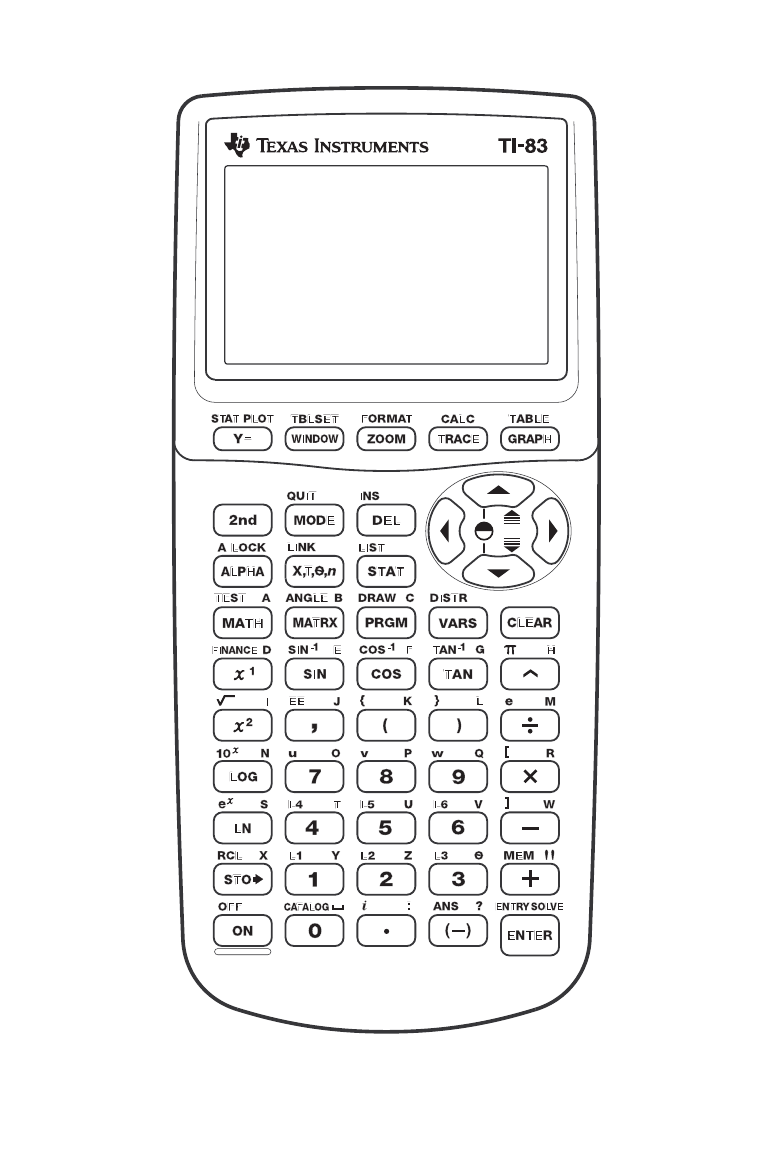
TI83CALC.DOC TI 83 Inside Cover Bob Fedorisko Revised: 12/03/99 8:31 AM Printed: 03/12/01 1:49
PM Page 1 of 2
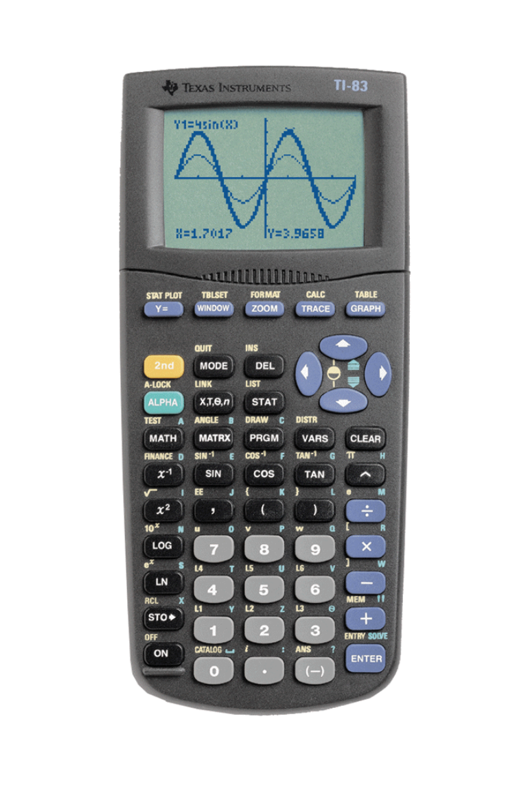
TI83CALC.DOC TI 83 Inside Cover Bob Fedorisko Revised: 12/03/99 8:31 AM Printed: 03/12/01 1:49
PM Page 2 of 2
